
RESEARCH ARTICLE
Kumaraswamy Distribution and Random Extrema
Tomasz J. Kozubowski1, *, Krzysztof Podgórski2
Article Information

Identifiers and Pagination:
Year: 2018Volume: 9
First Page: 18
Last Page: 25
Publisher Id: TOSPJ-9-18
DOI: 10.2174/1876527001809010017
Article History:
Received Date: 7/3/2018Revision Received Date: 26/6/2018
Acceptance Date: 29/6/2018
Electronic publication date: 31/7/2018
Collection year: 2018
open-access license: This is an open access article distributed under the terms of the Creative Commons Attribution 4.0 International Public License (CC-BY 4.0), a copy of which is available at: https://creativecommons.org/licenses/by/4.0/legalcode. This license permits unrestricted use, distribution, and reproduction in any medium, provided the original author and source are credited.
Abstract
Objective:
We provide a new stochastic representation for a Kumaraswamy random variable with arbitrary non-negative parameters. The representation is in terms of maxima and minima of independent distributed standard uniform components and extends a similar representation for integer-valued parameters.
Result:
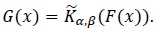
The result is further extended for generalized classes of distributions obtained from a “base” distribution function Fviz.G(x) = H(F(x)), where H is the CDF of Kumaraswamy distribution.
1. INTRODUCTION
There is a growing literature on generalized distributions based on Kumaraswamy distribution [1]. They are obtained from a “base” distribution with the cumulative distribution function (CDF) F as the CDF G (a generalized version of F) viz.
 |
(1) |
where
 |
(2) |
is the CDF of the Kumaraswamy distribution with parameters α, β > 0. The latter from now is denoted by Kα,β. In terms of random variables, the relation (1) can be stated as
 |
(3) |
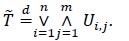
where Y~G and T~Kα,β. This generalization of F was proposed in Cordeiro and de Castro [2], where the authors developed its basic properties and presented generalizations of normal, Weibull, gamma, Gumbel, and inverse Gaussian distributions. Many other generalized distributions following this scheme have been developed since then, including recent works of de Pascoa et al. [3], Nadarajah et al. [4], Mameli [5] and Aryal and Zhang [6]. However, papers on the topic focus mainly on rather elementary properties and do not provide any significant theoretical interpretation of the construction. One exception is an interpretation for integer-valued α and β through maxima and minima of independent and identically distributed (IID) random components (e.g., Jones [7], Nadarajah et al. [4], Nadarajah and Eljabri [8]). Indeed, assuming that α = m, β = n are positive integers, we find that xm is the CDF of the maximum of m IID standard uniform variables, with the corresponding survivor function (SF) being 1 - xm. Thus, the quantity (1 - xm)n in (2) is the SF of the minimum of n such random variables, with H being the corresponding CDF. In other words, we have the following stochastic representation of T~Km,n,
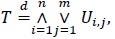 |
(4) |
where {Ui,j} are IID standard uniform variables. This property, discussed in Jones [7], motivated the name minimax for this distribution. Below we extend this interpretation to the general Kumaraswamy distribution as well as to its generalization (1).
2. MAIN RESULTS
To obtain a representation of a Kumaraswamy random variable in terms of min/max, we shall use the following basic result (e.g., Kozubowski and Podgórski, [9]), which relates the distributions of min/max of IID components with random number of terms to the relevant Probability Generating Function (PGF).
Lemma 2.1. If N is an  random variable, independent of the sequence {Xi} of IID random variables with the CDF F, then the CDFs of the random variables
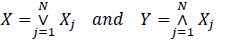 |
(5) |
are given by FX(x) = GN(F(x)) and FY(y) = 1 - GN(1 - F(y)) , respectively, where GN is the PGF of N.
A notable application of this result, discussed in Kozubowski and Podgórski [9], concerns a special case where the variable N = Nα in (5) has the Sibuya distribution (Sibuya, [10]), given by the PGF
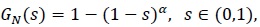 |
(6) |
and the Probability Mass Function (PMF)
 |
(7) |
where necessarily  , with the boundary case α = 1 corresponding to a unit mass at n = 1. This variable represents the number of trials till the first success in an infinite sequence of independent Bernoulli trials, where the probability of success varies with the trial, and for the nth trial equals α/n. Here, because of the special form of the PGF of the Sibuya random variable Nα, if the latter represents the random number of terms in Lemma 2.1, the CDFs of the random variables X and Y in (5) are given by FX(x) = 1 - [1 - F(x)]α and FY(Y) = [F(x)]α, respectively. This leads to our first result for the Kumaraswamy distribution with the parameters restricted to the unit interval (0, 1).
Proposition 2.1. Assume that {Ui,j} are IID standard uniform variables,  have Sibuya distributions with respective parameters
  , and all the variables on the right-hand-side of (8) are mutually independent. Then the variable
 |
(8) |
has the Kumaraswamy distribution Kα, β.
The above result can be re-formulated for any Kumaraswamy generalized random variable obtained viz. (3), providing a meaningful interpretation of this construction in terms of maxima and minima of IID components with the “parent” CDF F.
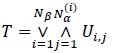
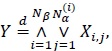
Proposition 2.2. Let Nα(i),  be IID Sibuya variables with parameter , and independent of another Sibuya variable Nβ, with parameter . Further, for a given CDF F, let Y be a random variable with the CDF G defined by (1), where H = Kα, β ; with
  . Then we have
 |
(9) |
where the {Xi,j} are IID random variables with CDF F, independent of Nα(i) and Nβ.
Remark 2.1. Let Bα, β denote beta distribution given by the PDF
 |
(10) |
Then, if either α = 1 or β = 1, the Kumaraswamy distribution Kα, β coincides with Bα, β. Thus, Proposition 2.1 specialized to this case, leads to stochastic representations of such beta-distributed random variables in terms of maxima and minima, i.e. if for the {Ui} are IID standard uniform random variables, independent of Sibuya-distributed Nα and Nβ with we define
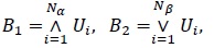 |
(11) |
then B1~Bα, 1 and B2~B1, β. Further, if either α = 1 or β = 1, the generalized distributions obtained viz. (1) are special cases of beta-generalized distributions popularized by Eugene et al. [11], arising when H in (1) is the CDF corresponding to (10). Thus, Proposition 2.2 specialized to this case shows that if a random variables Y is defined viz. (3), where either T~Bα, 1 or T~B1, β with , then we have
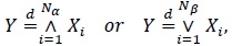 |
(12) |
respectively, where the {Xi} are IID random variables with CDF F, independent of Sibuya-distributed Nα and Nβ.
An extension of Proposition 2.1 to the case where the parameters are no longer restricted to the unit interval is straightforward. To formulate the result, we shall split a positive number r into r = {r} + < r >, where
 |
(13) |
We shall also need the following result taken from Kozubowski and Podgórski [9], where we use the standard convention that the min and max over an empty set are understood as ∞ and -∞, respectively.
Proposition 2.3. If X and Y have CDFs given by 1 - (1 - F(x))r and [F(x)]r, respectively, where F is a CDF and  , then they admit the stochastic representations
 |
(14) |
where N< r > has the Sibuya distribution (7) with parameter α = < r > and is independent of the IID {Xj} with the CDF F.
When we set r = β and apply the first representation in (14) to a Kumaraswamy random variable T~Kα, β, , we obtain
 |
(15) |
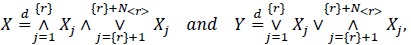
where N< β > has Sibuya distribution with parameter < β > and {Xj} is IID with the CDF xα. In turn, when we set r = α and apply the second representation in (14) to each Xj in (15), we obtain
 |
(16) |
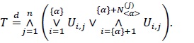
where the {Ui,j} are IID standard uniform variables and the N< α >(j) are IID and Sibuya distributed with parameter < α >, independent of the {Ui,j}. By combining (15) with (16), we obtain the following result.
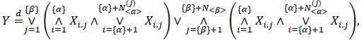
Proposition 2.4. Let T~Kα, β with general α, β > 0. Then we have
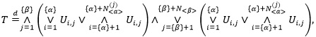 |
(17) |
where the {Ui,j} are IID standard uniform variables, N< α >(j) and N< β > have Sibuya distributions with respective parameters < α > and < β >, and all the variables on the right-hand-side of (17) are mutually independent.
Remark 2.2. If the parameter α of T~Kα, β is a positive integer,  , then we have {α} = m - 1, < α > = 1, so that the Sibuya variables N< α >(j) are equal to 1 almost surely. Thus, in the same notation, the representation (17) turns into
 |
(18) |
On the other hand, if the parameter β of T~Kα, β is a positive integer,  , then we have {β} = n - 1, < β > = 1, and the Sibuya variable N< β > is equal to 1 almost surely, in which case the representation (17) reduces to
 |
(19) |
Moreover, if both parameters of T~Kα, β are positive integers, so that in (18) we have and in (19) we have , then both, (18) and (19), turn into the representation (4) derived by Jones [7].
Remark 2.3. The stochastic representation (17) can be extended to the case of exponentiated Kumaraswamy (EK) distribution studied by Lemonte et al. [12], which is given by the CDF
 |
(20) |
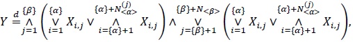
This can be achieved by another application of Proposition 2.3 on top of Proposition 2.4, leading to
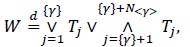 |
(21) |
where W has EK distribution (20), γ = {γ} + < γ > with 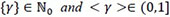 , and N< γ >has Sibuya distribution (7) with parameter α = < γ >, and is independent of the IID Kumaraswamy random variables {Tj} with the CDF (2). In turn, each of the Kumaraswamy variables Tj admits the stochastic representation (17) involving minima and maxima of IID standard uniform variables.
Finally, we extend Proposition 2.4 to generalized random variables obtained from Kumaraswamy distribution viz. (3), which links this construction with maxima and minima of IID components with the “parent” CDF F.
Proposition 2.5. Let Y be a random variable with the CDF G defined by (1), where H = Kα, β with α, β > 0. Then we have
 |
(22) |
where the {Xi,j} are IID random variables with CDF F, N< α >(j) and N< β > have Sibuya distributions with respective parameters < α > and < β >, and all variables on the right-hand-side of (22) are mutually independent.
Let us consider again the stochastic representation of T~Km, n given by (4). As discussed in Nadarajah et al. [4] (Nadarajah and Eljabri, [8]), T can be thought of as a lifetime of a system consisting of n sub-systems connected in a series, where each sub-system is composed of m IID components with standard uniform lifetimes. If the lifetimes are non-negative and IID with the CDF F, then similar interpretation holds for the random variable Y obtained viz. (3) with T~Km, n. The results presented above provide a similar interpretation for a general T~Kα, β as well as for a non-negative variable Y obtained viz. (3) with T~Kα, β, where the number of IID components is a random variable.
In connection with this interpretation of (4), one can instead assume that the n sub-systems are connected in parallel rather than in a series, while the IID standard uniform components {Ui,j} within each sub-system are connected in a series. In this case, the total lifetime of the system will admit the representation
 |
(23) |
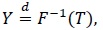
It is easy to see that  in (23) has the same distribution as 1 - T, where T~Km, n. More generally, let us consider the random variable
  , where T~Kα, β, which we shall call a dual of the latter, and denote its distribution by
  . Clearly,
 |
(24) |
Remark 2.4. Interestingly, the class of distributions on the unit interval defined viz. (24) coincides with the class of distributions whose CDFs are given by the quantile functions corresponding to the Kumaraswamy CDF (2).
All the results for the Kumaraswamy and Kumaraswamy-generated distributions presented above have analogs in terms of the dual distributions (24) and the generalizations of F obtained viz.
 |
(25) |
It turns out that they are obtained by swapping the minima with the maxima in the results for the Kumaraswamy and Kumaraswamy-generated distributions. We shall state them, without proofs, for distributions (25) since other results are obtained by setting F (x) = x. As before, we start with the case .
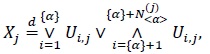
Proposition 2.6. Let F be a random variable with the CDF G defined by (25) with  have Sibuya distributions with respective parameters and . Then
 |
(26) |
where the {Xi,j} are IID random variables with CDF F, independent of the Sibuya variables.
An extension to the general case presented below can be derived from Proposition 2.3.
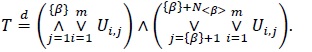
Proposition 2.7. Let Y be a random variable with the CDF G defined by (25) with α , β > 0. Then
 |
(27) |
where the {Xi,j} are IID random variables with CDF F, independent of two independent Sibuya variables N< α >(j) and N< β > with parameters < α > and < β >, respectively.
Remark 2.5. If Y in Propositions 2.6 and 2.7 has a dual Kumaraswamy distribution with the CDF (24), then the stochastic representations still apply with the {Xi,j} being IID standard uniform variables.
Remark 2.6. If the underlying variables are non-negative, our results have an interpretation in terms of series-parallel or parallel-series systems of IID components where the number of components can be random (and Sibuya distributed). For example, the quantity Y in Proposition 2.2 represents the lifetime of ra andom number Nβ of sub-systems connected in parallel, where each sub-system i consists of a random number Nα(i) of components connected in a series. Similarly, the quantity Y in Proposition 2.6 represents the lifetime of Nβ sub-systems connected in a series, where each sub-system consists of a random number of components connected in parallel. The other results have analogous, albeit not as straightforward, interpretations.
Remark 2.7. As discussed above, the stochastic representations for Kumaraswamy and related distributions are built on min/max interpretations of distributions given by the survival function  or the CDF Fr with non-negative r, where F is a “base” CDF. These two transformations are known as the proportional hazard and the proportional reversed hazard transforms (or models, see, e.g., Wang [13] and Di Crescenzo [14]), since the hazard rates of distributions given by F and are proportional (as are the the reversed hazard rates of distributions given by F and Fr). It also is worth noting that these two generalizations of F are examples of the so-called distorted distributions, which in general are obtained through a transformation q(F) where q is a continuous and increasing bijective function on the unit interval onto itself (see, e.g., Navarro et al. [15], Navarro [16], Navarro and Gomis [18] and references therein). Consequently, using this connection and the results for distorted distributions one can study preservation of reliability aging classes and related properties for Kumaraswamy-transformed distributions obtained viz. (1) or (25).
By means of Lemma 2.1, several other classes of generalized distributions based on a “parent” CDF F, which were introduced in recent years, can also be shown to arise from random maxima and minima of IID components with distribution F. For example, as shown by Kozubowski and Podgórski [18], if N has a Bernoulli distribution with parameter  shifted up by one, so that its PGF is
 |
(28) |
we obtain the so-called transmuted version of F, defined by
 |
(29) |
Another example is provided by the so-called Marschall-Olkin generalized-F distributions, which were made popular by Marshall and Olkin [19] who introduced them through minima and maxima of IID components (following distribution F) with a geometric number of terms N.
Remark 2.8. The CDF (29) is a generalized mixture of F and F2 (where the weights are allowed to be negative, see, e.g., Navarro, [16]) as well as usual mixture of F2 and 1 - (1 - F)2 (with non-negative weights (1 - α)/2 and (1 + α)/2, respectively). The latter representation as a mixed system (e.g., Samaniego, [20]) allows an alternative interpretation of (29) in terms of lifetimes of series/parallel systems with IID components.
CONSENT FOR PUBLICATION
Not applicable.
CONFLICT OF INTEREST
The authors declare no conflict of interest, financial or otherwise.
ACKNOWLEDGEMENTS
We thank two referees for their remarks and additional references. Kozubowski’s research was partially supported by the European Union’s Seventh Framework Programme for Research, Technological Development and Demonstration under grant agreement no 318984 - RARE. Podgórski’s research was supported by Swedish Research Council Grant Dnr: 2013-5180.