
RESEARCH ARTICLE
Comparing Different Information Levels
Uwe Saint-Mont*
Article Information

Identifiers and Pagination:
Year: 2017Volume: 8
First Page: 7
Last Page: 18
Publisher Id: TOSPJ-8-7
DOI: 10.2174/1876527001708010007
Article History:
Received Date: 06/03/2017Revision Received Date: 19/04/2017
Acceptance Date: 27/04/2017
Electronic publication date: 19/07/2017
Collection year: 2017
open-access license: This is an open access article distributed under the terms of the Creative Commons Attribution 4.0 International Public License (CC-BY 4.0), a copy of which is available at: https://creativecommons.org/licenses/by/4.0/legalcode. This license permits unrestricted use, distribution, and reproduction in any medium, provided the original author and source are credited.
Abstract
Objective:
Given a sequence of random variables X = X1, X2, . . .suppose the aim is to maximize one’s return by picking a ‘favorable’ Xi. Obviously, the expected payoff crucially depends on the information at hand. An optimally informed person knows all the values Xi = xi and thus receives E(sup Xi).
Method:
We will compare this return to the expected payoffs of a number of gamblers having less information, in particular supi(EXi), the value of the sequence to a person who only knows the random variables’ expected values.
In general, there is a stochastic environment, (F.E. a class of random variables C), and several levels of information. Given some XϵC, an observer possessing information j obtains rj(X). We are going to study ‘information sets’ of the form.
 |
characterizing the advantage of k relative to j. Since such a set measures the additional payoff by virtue of increased information, its analysis yields a number of interesting results, in particular ‘prophet-type’ inequalities.
1. SEVERAL INFORMATION LEVELS
Suppose there is a sequence of bounded random variables X = X1, X2, . . . and the aim is to maximize one’s return by picking a ‘favorable’ Xi. The first aim of this contribution is to study observers with different kinds of information:
Suppose an observer knows all the realizations of the random variables and may thus choose the largest one. His expected return is therefore
 |
(1) |
which is called the value to a prophet. Since the prophet always picks the largest realization his value m is a natural upper bound, given a sequence X.
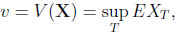
Traditionally, m has been compared to the value obtained by a statistician who observes the process sequentially. This gambler, studied in detail in Chow, Robbins & Sigmund (1971) [1], relies on stopping rules T, which have to be measurable with respect to the σ-field of past events. Behaving optimally the statistician may thus receive
 |
(2) |
If there is a finite horizon n, one defines v = supT  , T ≤n EXT and m = E(max1≤i≤n Xi).
To avoid trivialities, we assume n ≥ 2 throughout this article.
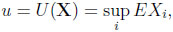
A minimally informed gambler has to make his choice on the basis that he only knows the random variables’ expected values. Behaving optimally, he gets
 |
(3) |
an amount that is entirely due to his (weak) prior information, and is a straightforward counterpart to E(supi Xi).
One might think that a person who knows the common distribution L(X1, . . ., Xn) (but none of the observations) should receive a larger payoff. However, no matter how this gambler makes up his mind, at the end of the day he has to choose an index i  {1, . . ., n}, and thus his expected reward will be largest if EXi = u. Thus, although he knows much more than the minimally informed gambler his superior knowledge does not pay off.
In other words, it’s the observations that make a difference. Suppose a person knows the dependence structure among the random variables and some of the observations, w.l.o.g. x1, . . ., xj . Notice, that there is no sequential unfolding of information, however, this partially informed gambler may use the values known to him to update his knowledge on the variables not observed, i.e. he may refer to conditional expectations.
Thus, he obtains
 |
and his expected return is
 |
(4) |
This observer can be reduced to a classical situation as follows: Given x1, . . ., xj , he will only consider the largest of these values; and the same with E(Xj+1|x1, . . ., xj ),..., E(Xn|x1, . . ., xj ). Thus w.l.o.g. it suffices to compare
 |
which is tantamount to the comparison of v and m if n = 2 and if arbitrary dependencies are allowed. In this situation the statistician behaves optimally if he chooses x1 whenever x1≥ E(X2|x1). Thus, the set of all possible values here is given by {(w,m)|w ≤ m ≤ 2w-w2, 0 ≤ w ≤ 1} if w.l.o.g. 0 ≤ Xi ≤ 1 for all i.
Stochastic Environments (Classes of Random Variables)
For some fixed X, the difference between two observers with different amounts of information can be nonexistent or arbitrarily large. In order to quantify the “value” of information it is thus necessary to shift attention to some class of random variables C, where M (X) is finite (and nonnegative) for all X C. It is then natural to consider the worst case scenarios. Traditionally these have been called prophet inequalities M (X) − V (X) ≤ a and M (X)/V (X) ≤ b with smallest possible constants a and b that hold for all X C.
Such stochastic inequalities follow easily from the more fundamental prophet region, that is,
 |
where fC is called the upper boundary function corresponding to C. Since it is only the latter set that gives a complete description of some informational advantage, it is more fundamental and should be considered in its own right.
In general, an information set characterizes the environment C, evaluated with the help of two particular levels of information. One could also prioritize the information edge and say that the difference between two levels of information (e.g., minimal vs. sequential), is studied in a certain environment. It is the second major aim of this article to illustrate a number of possible applications of these ideas.
2. MINIMAL VERSUS MAXIMUM INFORMATION
In this section we systematically compare u and m. That is, we are going to derive corresponding information sets (called prophet regions since m is involved) in two standard random environments: C(I, n), the class of all sequences of independent, [0, 1]- valued random variables with horizon n; and C(G, n), the class of all sequences of [0, 1]-valued random variables with horizon n.
Theorem 1(independent environment). LetX = (X1, . . ., Xn) C(I, n), U (X) = max EXi and M (X) = E(max Xi). Then the prophet region {(x, y) | x = U (X), y = M (X), X C(I, n)} is precisely the set
 |
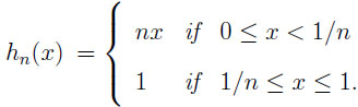
Theorem 2(general environment). LetX = (X1, . . ., Xn) C(G, n), U (X) = max EXi, and M (X) = E(max Xi). Then the upper boundary function hn of the prophet region is
is
 |
Proof of Theorem 1: Without loss of generality let x = EX1≥ max2≤i≤n EXi. Hill and Kertz [5] (1981: Lemma 2.2) prove that X can be replaced by a ‘dilated’ vector Y of Bernoulli random variables Y1, . . ., Yn such that EXi = EYi, 1 ≤ i ≤ n, and M (X) ≤ M (Y). Replacing Y by a vector of iid Bernoulli random variables Z = (Z1, . . ., Zn) such that EZi = x, 1 ≤ i ≤ n, does not improve the value to the gambler, i.e., U (X) = U (Y) = U (Z) = x, however, M (Y) ≤ M (Z) = 1 − (1 − x)n. Since any XC(I, n) can be replaced by a vector Z of iid Bernoulli random variables without changing the value to the gambler, fn(x) is the upper boundary function. Defining the independent random variables Z1', . . ., Zn' by means of P (Zi' = λ+(1−λ)x) = x/(λ+x−λx) = 1−P (Zi' = 0) and 0 ≤ λ ≤ 1 proves that all points between (x, x) and (x, 1 − (1 − x)n) also belong to the region. ♦
Notice that for every fixed x > 0, limn→∞ fn(x) ↑ 1 holds. Inspecting fn(x)/x and fn(x) − x immediately yields:
Corollary 1The prophet inequalities corresponding to C(I, n) are
 |
In the latter case,Z = (Z1, . . ., Zn) C(I, n) attains equality if the Zi are iid Bernoulli random variables such that U (Z) = EZi = P (Zi = 1) = 1 − n−1/(n−1).
Proof of Theorem 2: Denote by ei the i-th canonical unit vector. First consider the random variable Z = (Z1, . . ., Zn) having the distribution
| P (Z = e1) = . . . = P (Z = en) = 1/n. |
A minimally informed person picks any of the random variables Zi, which is 1 with probability 1/n and obtains U (Z) = 1/n. Since there is always exactly one i such that Zi = 1, whereas all the other random variables are zero, M (Z) = E(max Zi) = max1≤i≤n Zi ≡ 1.
To get a U (Z) ≥ 1/n, let P (Z = e1) = x ≥ 1/n and distribute the remaining probability equally among the other canonical unit vectors, i.e., P (Z = e2) = . . . = P (Z = en) = (1 − x)/(n − 1) ≤ x. Thus, the minimally informed observer may always pick the first random variable, giving him U (Z) = EZ1 = x and for the same reasons as before E(max Zi) = 1. Replacing ei by λei where 0 ≤ λ ≤ 1 and i = 2, . . ., n does not change the value to the gambler, but the value to the prophet decreases towards x if λ ↓ 0.
Finally, let X = (X1, . . ., Xn) C(G, n) and U (X) = x < 1/n. On the set Ai = {ω|Xi(ω) ≥ maxj,j≠i Xj (ω)} replace X(ω) = (X1(ω), . . ., Xn(ω)) by
Y(ω) = (0, . . ., 0, Xi(ω), 0, . . ., 0), i = 1, . . ., n. In the case of equality choose any component (e.g., the first) where the maximum is attained. Since Xi(ω) ≥ Yi(ω) we have U (X) = max EXi ≥ max EYi = U (Y) = y, and since max[X1(ω), . . ., Xn(ω)] = max[Y1(ω), . . ., Yn(ω)], M (X) = M (Y).
By construction, at most one component of Y(ω) is larger than zero. Thus max1≤i≤n Yi(ω) =  Yi(ω), and therefore
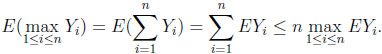 |
In the previous line equality is achieved if all expected values agree. Defining the distribution of Z = (Z1, . . ., Zn) via
| P (Z = e1) = . . . = P (Z = en) = y ≤ x < 1/n and P (Z = 0) = 1 − ny |
immediately yields U (Z) = y and M (Z) = ny. Since y may assume any value in the interval [0, 1/n) we have shown that hn(x) = nx is the upper boundary function if x < 1/n. A similar construction as before shows that all points between (x, x) and (x, nx) belong to the prophet region. ♦
An immediate consequence of the last theorem is:
Corollary 2The prophet inequalities corresponding to C(G, n) are M (X)/U (X) ≤ n and M (X)−U (X) ≤ 1−1/n. In the latter case equality is attained by P (Z = ei) = 1/n, (i = 1, . . ., n) where ei denotes the i-th canonical unit vector.
Remark. Although we focus on the prophet, other comparisons, in particular involving the statistician, would be interesting too. Comparing u and v for example, reveals the difference between prior information on the one hand and additional acquired information (sequential observations) on the other.
3. APPLYING INFORMATION SETS
In this section we restrict attention to classical prophet-statistician comparisons (vvs.m). However, the same kind of systematic analysis could be performed on any random environment and observers with different levels of information. An example will be given in the last section where we will compare u an m.
3.1. Some Well-Known Results
To illustrate how information sets may be used, we first collect a number of well-known results. To this end we introduce further random environments: Ciid, the class of all sequences of iid, [0, 1]-valued random variables; CI , the class of all sequences of independent, [0, 1]-valued random variables; CG, the class of all sequences of [0, 1]- valued random variables, and their corresponding counterparts with finite horizon, i.e., Ciidn, CIn = C(I, n), and CGn = C(G, n).
The β-discounted environment Cβ is defined by X1 = Y1, X2 = βY2, X3 = β2Y3, . . ., (0 ≤ β ≤ 1) and Y = (Y1, Y2, . . .) CI . Closely related are random variables X1, . . ., Xn with “increasing bounds”, i.e., ai ≤ Xi ≤ bi and nondecreasing sequences (ai) and (bi). In both cases it suffices to study n = 2, i.e., X1 = αY1, X2 = Y2 and X1 = Y1, X2 = βY2, respectively, where α, β [0, 1], and (Y1, Y2) CI2.
The following table collects a number of well-known “prophet” results, i.e., systematic comparisons of v and m (see Hill and Kertz (1983), Hill (1983), Kertz (1986), Boshuizen (1991), and Saint-Mont (1998)) [2, 3, 4], [6-9]:
| Random Environment | Upper boundary function |
|---|---|
|
CG CGn |
fG(x) = x − x ln(x) gn(x) = nx − (n − 1) xn/(n−1) |
|
Ciid Ciidn |
x φn(x) strictly increasing, strictly concave, differentiable |
| CI, CIn | fI (x) = 2x − x2 |
| Cαn | 2x − x2 if x < α; and x + (1 − x)α if x ≥ α |
| Cβ, Cβn |
fβ (x) = 2x − x2/β if x < 1 −  , and , andfβ (x) = x + (1 − x)(2(1 − ) − β) if x ≥ 1 − √1 −
|
In general, the difficult part consists in finding an upper boundary function, yet it is easy to show that all pairs (x, y) with x ≤ y < fC (x) belong to some prophet region. Moreover, prophet inequalities follow straightforwardly from prophet regions. As an example, look at RI : Since fI (x)/x = 2 − x ≤ 2 and fI (x) − x = x(1 − x) ≤ 1/4, we have M (X)/V (X) ≤ 2 and M (X) − V (X) ≤ 1/4 for all XCI . The same kind of argument yields M (X) < V (X)(1 − ln V (X)) and M (X) − V (X) < 1/e for all XCG.
3.2. Graphical Comparisons
What can be learned from this upon comparing two observers with different information levels? For every fixed horizon n, we have Riidn RInRGn. It also turns out that Riidn
 Riidm and RGnRGm whenever n < m. Thus the longer the horizon or the more general the environment, the better the outcome for the prophet (or the better informed person in general). On the other hand, restrictions of any kind, in particular the range of the random variables, makes the corresponding prophet (or information) region smaller. For example, Rα2 and Rβ must be subsets of RI .
The following illustration combines results achieved so far.
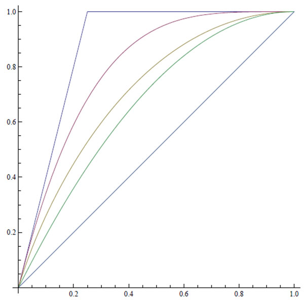 |
Illustration 1. From above: The functions h4(x), f4(x), g4(x), fI (x), and x.
Note that h4 and f4 stem from comparisons of u and m, whereas g4 and fI are the result of comparisons of v and m in the general and the independent environments, respectively.
Since for any environment RCv,mRCu,m, we must have g4≤ h4 and fI ≤ f4. In the case n = 2, the functions fI and f2 agree. This is no coincidence since X1≡ x and x = P (X2 = 1) = 1 − P (X2 = 0) is the (standard) worst case scenario for the statistician, and x = P (Xi = 1) = 1 − P (Xi = 0), (i = 1, 2) is the worst case scenario for the minimally informed gambler considered above. In both scenarios their values, v and u, respectively, agree (e.g., the obervers may both choose the second random variable) giving the prophet a maximum advantage of x(1 − x).
3.3. The Overall Information Difference
The diagonal ‘y = x’ collects all situations where the information edge of a better informed person does not result in a larger payoff. Thus, a degenerated prophet region indicates that given a stochastic environment the information lead of the prophet never pays off. Yet, the further some upper boundary function is away from the identical function, the larger the better-informed gambler’s overall advantage. A natural measure of this advantage is the area between these functions, i.e., the integral
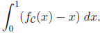 |
Given CI, the prophet’s advantage is qI =  x (1 – x) dx = 1/6. In the discounted environment, after some algebra, we obtain
 |
Note that q(1) = aI = 1/6, and l‘Hopital’s rule gives limβ↓0 0q(β) = 0. Moreover, q(β) is a convex function.
In the “increasing bounds” environment, after a little algebra, we obtain
 |
Note that  (1) = qI = 1/6, and l‘Hopital’s rule gives limα↓0 0(α) = 0. Moreover, (α) is a concave function.
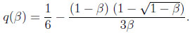
Illustration 2.α and β are shown on the x-axis. The functions on the unit interval from the top down are the constant qI = 1/6, (α) and q(β). The vertical and the horizontal lines will be explained in Section 3.5.
 |
However, given C(G, n), qI is augmented to
 |
In particular, qG(2) = 1/6, qG(3) = 1/5, qG(4) = 3/14, qG(5) = 2/9, and qG(6) = 5/22. Moreover, qG(n) is strictly increasing in n with limit 1/4, and
 |
3.4. Inverse Problems
Given a stochastic environment C, the standard interpretation of a prophet inequality is to look for a value to the statistician x0 = V (X), such that the difference fC (x) − x is maximized. In the same vein one may look for a value y0 on the y-axis, where the difference between the upper boundary and the identical function is at its greatest point. In the independent case this amounts to inverting fI (x) = 2x−x2, which yields f −1(y) = 1− . Maximizing y−(1 −) gives 1/4, which is obtained for y0 = 3/4.
Why do both perspectives agree with respect to the maximum difference? The reason is that the statement M (X) − V (X) ≤ 1/4 holds for all XCI , and thus is a property of the stochastic environment (and the two levels of information considered). The pair (1/2, 3/4) RI is a point in two-dimensional space, attained by certain extremal sequences X*. Thus, no matter how we choose to look at some region RC , the corresponding prophet inequalities must hold.
However, the analytic considerations involving the inverse of the upper boundary function may be quite different. In the discounted case, fβ-1(y) = β(1 − ) if y ≤ g(1 − ) = 3 − 2/β − 2 + 2/β = y(β). Otherwise, it is easily seen that
  is a linear, strictly decreasing function of y, and (1) = 1. The maximum of the function y − β(1 −) occurs at the point y = 3β/4 and is β/4.
Notice that,
 |
Thus, 3β/4 < y(β) for all β > 0. Due to continuity of , this yields β/4 as the overall maximum of the difference, always occurring at y = 3β/4. Traditionally, one would have said that the maximum difference of β/4 occurs at x = β/2.
Given CG, one has to invert fG(x) = x − x ln(x) in the unit interval. Using the theorem of the derivative of the inverse function, one may check that exp(1 + W−1(−y/e)) is the inverse, where W−1(y) is the lower real branch of the Lambert function (see Corless, Gonnet, Hare & Jeffrey 1996: 331). Thus (y − exp(1 + W−1(−y/e)))' = 1 + 1/(1 + W-1 (−y/e)) and W (−2/e2) = −2 immediately yield that the maximum occurs at y = 2/e and equals 1/e. Traditionally, it’s the same difference occuring at x = 1/e.
3.5. Comparing Stochastic Environments
Switching stochastic environments amounts to a systematic comparison of the associated regions. In particular, if  is less general than
  , we have R R . Obviously, it suffices to consider the upper boundary functions f, f of the two environments involved. Traditionally, one would only determine supx(f (x) − f(x)). However, in the inverse problem, supy (
 (y) ‒ (y)), and the area (f(x) − f (x)) dx are also natural measures of discrepancy.
To illustrate the above, let us compare CI and CG:
First, (fG(x) ‒ fI (x)) dx = 3/4 ‒ 2/3 = 1/12.
Second, maximizing d'(x) = fG(x) − fI (x) = x2− x − x ln x leads to d' (x) = 0  2x−ln x = 2, which has the explicit solution x0 = −W0 (−2/e2)/2 ≈ 0, 406376/2, where W 0 is the principal (upper) real branch of the Lambert W function (see Corless, Gonnet, Hare & Jeffrey 1996: 331). The point (x0 , d(x0 )) ≈ (0.2, 0.162) may be interpreted as follows: For every value x to the statistician, fI (x) is the best a prophet can obtain in the independent environment CI , and he can get arbitrary close to fG(x) if he is confronted with the general environment CG. Given x, the difference fG(x) − fI (x) reflects the additional gain (almost) obtainable to the prophet when moving from CI to CG, i.e., from the restricted to the more general situation. The additional sequences of random variables provide him with an additional reward of d(x) = x(x − ln x − 1), which is maximized if x = −W0 (−2/e2)/2, yielding 0.162 as the additional payoff.
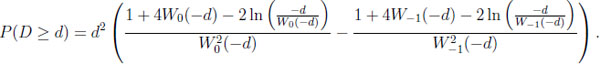
Third, starting with the prophet, the difference to be considered is δ(y) =  (y) ‒
(y) ‒  (y) = 1 ‒ ‒ exp(1+W-1 (‒y/e)). Thus, conditional on y, the statistician may (almost) lose this amount when the stochastic environment switches from independent to arbitrary sequences of random variables. Determining the value y0 where δ(y) is at its greatest, means looking for a constellation where the loss occurring to the statistician is the most pronounced when moving from CI to CG. Now δ'(y) = 0 is equivalent to finding the unique root of the equation,
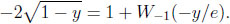 |
As a function of y, both the left hand side (L) and the right hand side (R) of the equation are twice differentiable. On the unit interval L(y) is convex, strictly increasing, L(0) = −2, and L(1) = 0. R(y) is concave, strictly increasing, limy↓0 R(y) = −∞, and R(0) = 0. Numerically, this yields the solution (y0 , δ(y0 )) ≈ (0.70, 0.119). Thus, in the worst case, the statistician loses about 0.119, which is considerably less than the prophet can hope to obtain when the environment extends from CI to CG.
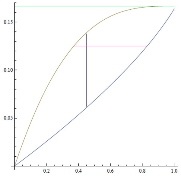
The next illustration summarizes these results:
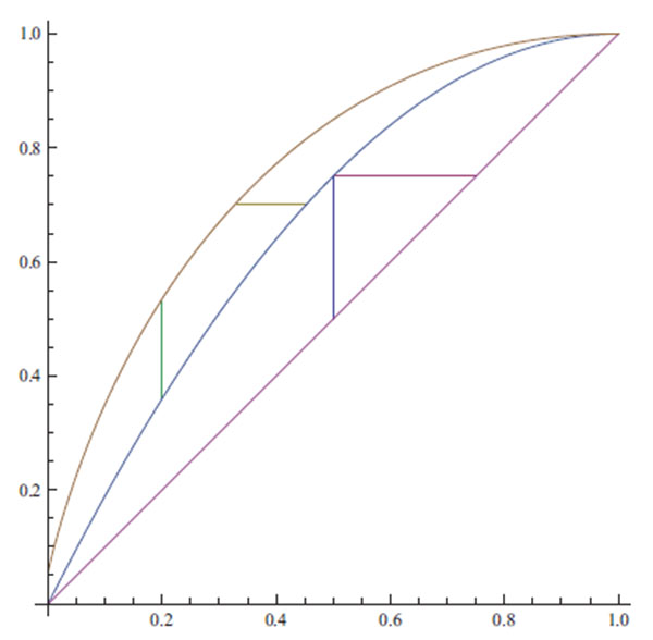 |
Illustration 3. From above: The functions fG, fI , and x on the unit interval. The small vertical line to the left illustrates the position of the maximum of the function d(x), the small horizontal line illustrates the maximum of the function δ(y), details in text. The other lines indicate the position of the maximum difference between the statistician and the prophet in the independent environment, see the second paragraph of Section 3.4.
A different kind of analysis may be explicated using the regions Cα2 and Cβ2: Illustration 2 points out that restricting the range of the second random variable (β-discounting), always produces a smaller region than restricting the range of the first random variable by the same amount α. On the one hand, the largest difference between the size of the regions occurs if α = β ≈ 0.45 and is approximately 0.077. On the other hand, suppose that the areas of Rα and Rβ agree. This is tantamount to fixing a point on the y-axis. In this case the largest difference between the parameter values occurs if the area covered by each of the regions is about 1/8. There, α ≈ 0.38 and β ≈ 0.83, thus the largest difference between the parameter values is approximately 0.452.
Of course, analyses along the same lines can be carried out for other regions, e.g., RI and Riidn, Riidn and Riidn+1, RGn and RGn+1, or RGn and RG.
3.6. Typical Differences and Ratios
Classical prophet inequalities are ‘worst case’ scenarios. They refer to the maximum advantage of the prophet over the statistician. Additionally, it is straightforward to ask for a ‘typical’ advantage, in particular a ‘typical’ difference or ratio. To do so, one would have to define a probability measure on some environment C. Since the classes of random variables considered are rather large, it is by no means clear how to do so in a natural way. However, starting with a stochastic environment and two distinguished levels of information, it is natural to consider the uniform measure on the corresponding prophet region RC .
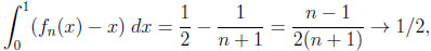
Given the independent environment, the size of RI is 1/6. Thus, we obtain as the typical difference between M (X) and V (X)
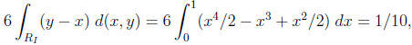 |
instead of 1/4 in the worst case. Moreover, the typical ratio is
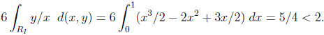 |
Given CG, RG covers an area of 1/4, giving the following typical difference and ratio:
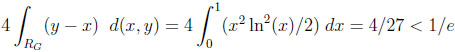 |
and
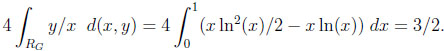 |
The last equation is particularly interesting, since there is no upper bound in the corresponding worst case scenario. Notice in the other examples that the typical results are considerably smaller than the constants in the corresponding worst cases.
Moreover, one may ask about the probability that a typical difference or ratio exceeds a certain bound. The ratio y/x = c y = cx is a straight line through the origin, so, given CI , the question amounts to calculating
 |
where t = 2 − c ≥ 0 is determined by the equation cx = y = 2x − x2, and 1 ≤ c ≤ 2.
Given CG, we obtain
 |
where t is determined by the equation cx = x − x ln x t = exp(1 − c), and c ≥ 1.
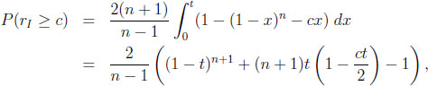
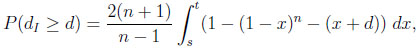
In the case of the difference, we are interested in the probability that it exceeds a certain bound d ≥ 0. Again, consider CI first. Since y −x = d y = x+d, we have to calculate
 |
Here, 0 ≤ d ≤ 1/4, and s and t are determined by the roots of the equation x + d = 2x − x2 in the unit interval, that is, s = 1/2- and t = 1/2 + .
Finally, given CG, we obtain with 0 ≤ d ≤ 1/e
 |
where s and t are determined by the roots of the equation d = −x ln x in the unit interval. Some algebra is needed to get s = exp(W−1(−d)) and t = exp(W0 (−d)). The subsequent integration results in
 |
4. A SYSTEMATIC STUDY OF THE NEW INFORMATION SETS
In the following we are going to apply the 'program' outlined in the last section to u and m, using the independent and the general stochastic environments.
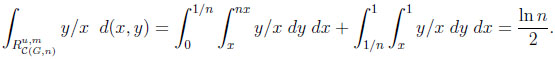
The overall information difference. Let us first compute the areas of  ,
,
 |
and  .
.
 |
Thus, their overall information distance is the size of the set \,
 |
Inverse Problems. In the independent case,  (y) = 1 ‒
  is the inverse function. The maximum of y ‒ (1 ‒ ) is attained for y0 = 1 − n−n/(n−1) and equals n−1/(n−1)− n−n/(n−1). In the general case, the inverse function is hn−1(y) = y/n. Thus, the maximum of y − y/n is attained at y0 = 1, giving a maximum difference of 1 − 1/n.
Comparing the independent and the general environments. Here, one has to maximize d(x) = (1 − x)n + nx − 1. Since d' (x) = n(1 − (1 − x)n−1) > 0 if x ≤ 1/n, the maximum occurs at x0 = 1/n and yields a difference of (1 − 1/n)n, converging to 1/e if n → ∞. The inverse functions lead to a difference of δ(y) = 1 − (1 − y)1/n − y/n. Thus, δ' (y) = −(1 − (1 − y)(n−1)/−n)/n > 0 if y > 0, and the maximum occurs at y0 = 1, yielding a difference of 1 − 1/n.
Typical differences and ratios. For CIn we calculate
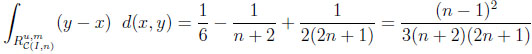 |
and
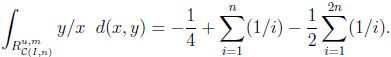 |
Thus, the typical difference dI and the typical ratio rI in the independent situation are
 |
For CGn , analogous integrations yield
 |
and
 |
Thus, the typical difference dG and the typical ratio rG in the general environment are
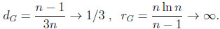 |
Probabilities that a typical difference or ratio exceeds a certain bound. For 1 ≤ c ≤ n this amounts to calculating
 |
where t is the unique root of the equation cx = 1 − (1 − x)n in the unit interval, and
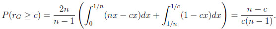 |
Notice that limn→∞(n − c)/(c(n − 1)) = 1/c.
In the case of the difference, given CIn, and thus 0 ≤ d ≤ n−1/(n−1)− n−n/(n−1), we calculate
 |
where the values of s and t (s < t) are determined by the roots of the equation x + d = 1 − (1 − x)n in the unit interval. Again, in general, s and t cannot be given explicitly. Finally, given CGn , we obtain with 0 ≤ d ≤ 1 − 1/n
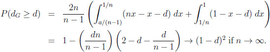 |
In both cases the prophet regions and converge towards the upper triangle T = {(x, y)|0 ≤ x ≤ y ≤ 1} in the unit square. Thus, in the limit, the typical ratios and differences agree and can be computed directly via T, yielding the probabilities 1/c and (1 − d)2.
CONSENT FOR PUBLICATION
Not applicable.
CONFLICT OF INTEREST
The author declares no conflict of interest, financial or otherwise.
ACKNOWLEDGEMENTS
Declared none.