
RESEARCH ARTICLE
A New Acceptance Sampling Plans Based on Percentiles for Odds Exponential Log Logistic Distribution
G.S. Rao1, *, K. Rosaiah2, K. Kalyani3, D.C.U. Sivakumar3
Article Information

Identifiers and Pagination:
Year: 2016Volume: 7
First Page: 45
Last Page: 52
Publisher Id: TOSPJ-7-45
DOI: 10.2174/1876527001607010045
Article History:
Received Date: 24/05/2016Revision Received Date: 08/09/2016
Acceptance Date: 23/09/2016
Electronic publication date: 30/11/2016
Collection year: 2016
open-access license: This is an open access article licensed under the terms of the Creative Commons Attribution-Non-Commercial 4.0 International Public License (CC BY-NC 4.0) (https://creativecommons.org/licenses/by-nc/4.0/legalcode), which permits unrestricted, non-commercial use, distribution and reproduction in any medium, provided the work is properly cited.
Abstract
In this paper, acceptance sampling plans are developed for the odds exponential log logistic distribution (OELLD) introduced by Rosaiah et al. [1] based on lifetime percentiles when the life test is truncated at a predetermined time. The minimum sample size necessary to ensure the specified lifetime percentile is obtained under a given customer’s risk. The operating characteristic values of the sampling plans as well as the producer’s risk are presented. One example with real data set is also given as an illustration.
1. INTRODUCTION
In most of the statistical quality control experiment, it is not possible to perform 100% inspection due to various reasons. The acceptance sampling plans are concerned with accepting or rejecting a submitted lot of a large size of products on the basis of the quality of the products inspected in a sample taken from the lot. An acceptance sampling plan is a specified plan that establishes the minimum sample size to be used for testing. In most acceptance sampling plans for a truncated life test, the major issue is to determine the sample size from a lot under consideration. Traditionally, when the life test indicates that the mean life of products exceeds the specified one, the lot of products is accepted, otherwise it is rejected. For the purpose of reducing the test time and cost, a truncated life test may be conducted to determine the smallest sample size to ensure a certain mean life time/percentile life time of products when the life test is terminated at a time, t0 and the number of failures observed does not exceed a given acceptance number c.
A common practice in life testing is to terminate the life test by a predetermined time t0 and note the number of failures. One of the objectives of these experiments is to set a lower confidence limit on the mean life/percentile lifetime. It is then to establish a specified mean life with a given probability, which provides protection to consumers. The test may be terminated before the time is reached or when the number of failures exceeds the acceptance number c in which case the decision is to reject the lot.
In the literature of acceptance sampling, there are many methods of testing. Epstein [2] was the first who considered truncated life tests in the exponential distribution. Truncated life tests are considered by many authors for various distributions: for example Sobel and Tischendrof [3], Gupta and Groll [4], Kantam and Rosaiah [5], Baklizi and El Masri [6], Tsai and Wu [7], Balakrishnan et al. [8], Kantam et al. [9], Rao et al. [10] and the references there in.
The above authors considered the design of acceptance sampling plans based on the population mean under a truncated life test. Gupta [11] suggested that for a skewed distribution the median represents a better quality parameter than the mean. On the other hand, for a symmetric distribution, mean is preferable to use as a quality parameter. Lio et al. [12, 13] considered acceptance sampling plans based on the truncated life tests to Birnbaum-Saunders distribution and Burr type XII for percentiles and they proposed that the acceptance sampling plans based on mean may not satisfy the requirement of engineering on the specific percentile of strength or breaking stress. When the quality of a specified low percentile is concerned, the acceptance sampling plans based on the population mean could pass a lot which has the low percentile below the required standard of consumers. Furthermore, a small decrease in the mean with a simultaneous small increase in the variance can result in a significant downward shift in small percentiles of interest. This means that a lot of products could be accepted due to a small decrease in the mean life after inspection. But the material strengths of products are deteriorated significantly and may not meet the consumer’s expectation. Therefore, engineers pay more attention to the percentiles of lifetime than the mean life in life testing applications. Moreover, most of the employed life distributions are not symmetric. Actually, percentiles provide more information regarding a life distribution than the mean life does. When the life distribution is symmetric, the 50th percentile or the median is equivalent to the mean life. Hence, developing acceptance sampling plans based on percentiles of a life distribution can be treated as a generalization of developing acceptance sampling plans based on the mean life of items. Balakrishnan et al. [8] proposed the acceptance sampling plans could be used for the quantiles and derived the formulae whereas Lio et al. [12, 13] developed for the acceptance sampling plans for any other percentiles of the Birnbaum-Saunders (BS) and Burr Type XII models. They have developed the acceptance sampling plans for percentile by replacing the scale parameter by the 100qth percentile. Rao and Kantam [14] and Rao et al. [15] developed acceptance sampling plans from truncated life tests based on the log-logistic and inverse Rayleigh distributions for Percentiles. Rao et al. [16] developed acceptance sampling plans for percentiles assuming linear failure rate distribution. Balamurali et al. [17] developed acceptance sampling plans based on median life for Fréchet distribution. These reasons motivate to develop acceptance sampling plans based on the percentiles, since odds exponential log logistic distribution (OELLD) is a skewed distribution, we prefer to use the percentile point as the quality parameter, and it will be denoted by. The rest of the paper is organized as follows. In Section 2, we describe concisely the OELLD. The design of proposed acceptance sampling plan for lifetime percentiles under a truncated life test is discussed in Section 3. In Section 4, we present the description of the proposed plan and obtain the necessary results. An example with real data set is also given as an illustration. Finally, conclusions are made in Section 5.
| β | δ=1.0 | δ=1.5 | δ=2 | δ=2.5 | |||||||||
|---|---|---|---|---|---|---|---|---|---|---|---|---|---|
| c | n | c | n | c | n | c | n | ||||||
| 0.25 | 2 | 6 | 16 | 0.9594 | 7 | 12 | 0.9683 | 8 | 11 | 0.9673 | 9 | 11 | 0.9595 |
| 4 | 2 | 7 | 0.9845 | 2 | 5 | 0.9748 | 2 | 4 | 0.9656 | 2 | 3 | 0.9756 | |
| 6 | 1 | 5 | 0.9807 | 1 | 3 | 0.9805 | 1 | 3 | 0.9571 | 1 | 2 | 0.9711 | |
| 8 | 1 | 5 | 0.9914 | 1 | 3 | 0.9913 | 1 | 3 | 0.9805 | 1 | 2 | 0.9870 | |
| 10 | 0 | 2 | 0.9571 | 1 | 3 | 0.9954 | 1 | 3 | 0.9896 | 1 | 2 | 0.9931 | |
| 0.10 | 2 | 9 | 26 | 0.9604 | 9 | 17 | 0.9514 | 9 | 13 | 0.9539 | 12 | 15 | 0.9616 |
| 4 | 2 | 9 | 0.9672 | 2 | 6 | 0.9550 | 2 | 4 | 0.9656 | 3 | 5 | 0.9728 | |
| 6 | 1 | 7 | 0.9618 | 1 | 4 | 0.9631 | 1 | 3 | 0.9571 | 2 | 4 | 0.9828 | |
| 8 | 1 | 7 | 0.9827 | 1 | 4 | 0.9833 | 1 | 3 | 0.9805 | 1 | 3 | 0.9639 | |
| 10 | 1 | 7 | 0.9908 | 1 | 4 | 0.9911 | 1 | 3 | 0.9896 | 1 | 3 | 0.9805 | |
| 0.05 | 2 | 10 | 30 | 0.9552 | 11 | 21 | 0.9588 | 12 | 18 | 0.9519 | 14 | 18 | 0.9525 |
| 4 | 3 | 13 | 0.9816 | 3 | 8 | 0.9800 | 3 | 6 | 0.9771 | 3 | 5 | 0.9728 | |
| 6 | 1 | 8 | 0.9506 | 2 | 7 | 0.9845 | 2 | 5 | 0.9840 | 2 | 4 | 0.9828 | |
| 8 | 1 | 8 | 0.9774 | 1 | 5 | 0.9732 | 1 | 4 | 0.9631 | 1 | 3 | 0.9640 | |
| 10 | 1 | 8 | 0.9879 | 1 | 5 | 0.9856 | 1 | 4 | 0.9800 | 1 | 3 | 0.9805 | |
| 0.01 | 2 | 14 | 45 | 0.9511 | - | - | - | - | - | - | - | - | - |
| 4 | 3 | 17 | 0.9530 | 3 | 10 | 0.9530 | 3 | 7 | 0.9557 | 4 | 7 | 0.9752 | |
| 6 | 2 | 14 | 0.9757 | 2 | 8 | 0.9767 | 2 | 6 | 0.9709 | 2 | 5 | 0.9625 | |
| 8 | 1 | 11 | 0.9582 | 1 | 6 | 0.9612 | 1 | 4 | 0.9631 | 2 | 5 | 0.9876 | |
| 10 | 1 | 11 | 0.9773 | 1 | 6 | 0.9790 | 1 | 4 | 0.9800 | 1 | 4 | 0.9631 | |
| β | δ=1.0 | δ=1.5 | δ=2 | δ=2.5 | |||||||||
|---|---|---|---|---|---|---|---|---|---|---|---|---|---|
| c | n | c | n | c | n | c | n | ||||||
| 0.25 | 2 | 6 | 16 | 0.9594 | 7 | 12 | 0.9683 | 8 | 11 | 0.9673 | 9 | 11 | 0.9595 |
| 4 | 2 | 7 | 0.9845 | 2 | 5 | 0.9748 | 2 | 4 | 0.9656 | 2 | 3 | 0.9756 | |
| 6 | 1 | 5 | 0.9807 | 1 | 3 | 0.9805 | 1 | 3 | 0.9571 | 1 | 2 | 0.9711 | |
| 8 | 1 | 5 | 0.9914 | 1 | 3 | 0.9913 | 1 | 3 | 0.9805 | 1 | 2 | 0.9870 | |
| 10 | 0 | 2 | 0.9571 | 1 | 3 | 0.9954 | 1 | 3 | 0.9896 | 1 | 2 | 0.9931 | |
| 0.1 | 2 | 9 | 26 | 0.9604 | 9 | 17 | 0.9514 | 9 | 13 | 0.9539 | 12 | 15 | 0.9616 |
| 4 | 2 | 9 | 0.9672 | 2 | 6 | 0.9550 | 2 | 4 | 0.9656 | 3 | 5 | 0.9728 | |
| 6 | 1 | 7 | 0.9618 | 1 | 4 | 0.9631 | 1 | 3 | 0.9571 | 2 | 4 | 0.9828 | |
| 8 | 1 | 7 | 0.9827 | 1 | 4 | 0.9833 | 1 | 3 | 0.9805 | 1 | 3 | 0.9639 | |
| 10 | 1 | 7 | 0.9908 | 1 | 4 | 0.9911 | 1 | 3 | 0.9896 | 1 | 3 | 0.9805 | |
| 0.05 | 2 | 10 | 30 | 0.9552 | 11 | 21 | 0.9588 | 12 | 18 | 0.9519 | 14 | 18 | 0.9525 |
| 4 | 3 | 13 | 0.9816 | 3 | 8 | 0.9800 | 3 | 6 | 0.9771 | 3 | 5 | 0.9728 | |
| 6 | 1 | 8 | 0.9506 | 2 | 7 | 0.9845 | 2 | 5 | 0.9840 | 2 | 4 | 0.9828 | |
| 8 | 1 | 8 | 0.9774 | 1 | 5 | 0.9732 | 1 | 4 | 0.9631 | 1 | 3 | 0.9639 | |
| 10 | 1 | 8 | 0.9879 | 1 | 5 | 0.9856 | 1 | 4 | 0.9800 | 1 | 3 | 0.9805 | |
| 0.01 | 2 | 14 | 45 | 0.9511 | - | - | - | - | - | - | - | - | - |
| 4 | 3 | 17 | 0.9530 | 3 | 10 | 0.9530 | 3 | 7 | 0.9557 | 4 | 7 | 0.9752 | |
| 6 | 2 | 14 | 0.9757 | 2 | 8 | 0.9767 | 2 | 6 | 0.9709 | 2 | 5 | 0.9625 | |
| 8 | 1 | 11 | 0.9582 | 1 | 6 | 0.9612 | 1 | 4 | 0.9631 | 2 | 5 | 0.9876 | |
| 10 | 1 | 11 | 0.9773 | 1 | 6 | 0.9790 | 1 | 4 | 0.9800 | 1 | 4 | 0.9631 | |
| β | δ=1.0 | δ=1.5 | δ=2 | δ=2.5 | |||||||||
|---|---|---|---|---|---|---|---|---|---|---|---|---|---|
| c | n | c | n | c | n | c | n | ||||||
| 0.25 | 2 | 4 | 12 | 0.9697 | 4 | 7 | 0.9605 | 6 | 8 | 0.9648 | 7 | 8 | 0.9634 |
| 4 | 1 | 5 | 0.9835 | 1 | 3 | 0.9757 | 1 | 2 | 0.9747 | 2 | 3 | 0.9867 | |
| 6 | 0 | 2 | 0.9622 | 0 | 1 | 0.9576 | 1 | 2 | 0.9945 | 1 | 2 | 0.9871 | |
| 8 | 0 | 2 | 0.9786 | 0 | 1 | 0.9759 | 0 | 1 | 0.9576 | 1 | 2 | 0.9957 | |
| 10 | 0 | 2 | 0.9862 | 0 | 1 | 0.9845 | 0 | 1 | 0.9727 | 0 | 1 | 0.9576 | |
| 0.10 | 2 | 5 | 17 | 0.9587 | 5 | 9 | 0.9637 | 6 | 8 | 0.9648 | 11 | 13 | 0.9645 |
| 4 | 1 | 7 | 0.9673 | 1 | 4 | 0.9544 | 2 | 4 | 0.9858 | 2 | 3 | 0.9867 | |
| 6 | 1 | 7 | 0.9928 | 1 | 4 | 0.9898 | 1 | 3 | 0.9843 | 1 | 2 | 0.9871 | |
| 8 | 0 | 4 | 0.9576 | 0 | 2 | 0.9524 | 0 | 1 | 0.9576 | 1 | 2 | 0.9957 | |
| 10 | 0 | 4 | 0.9727 | 0 | 2 | 0.9693 | 0 | 1 | 0.9727 | 0 | 1 | 0.9576 | |
| 0.05 | 2 | 6 | 21 | 0.9616 | 7 | 13 | 0.9714 | 8 | 11 | 0.9673 | 11 | 13 | 0.9645 |
| 4 | 1 | 8 | 0.9576 | 1 | 4 | 0.9544 | 2 | 4 | 0.9858 | 2 | 3 | 0.9867 | |
| 6 | 1 | 8 | 0.9906 | 1 | 4 | 0.9898 | 1 | 3 | 0.9843 | 1 | 2 | 0.9871 | |
| 8 | 1 | 8 | 0.9969 | 0 | 2 | 0.9524 | 1 | 3 | 0.9948 | 1 | 2 | 0.9957 | |
| 10 | 0 | 5 | 0.9659 | 0 | 2 | 0.9693 | 1 | 3 | 0.9978 | 0 | 1 | 0.9576 | |
| 0.01 | 2 | 8 | 30 | 0.961 | 8 | 16 | 0.959 | 9 | 13 | 0.9539 | 14 | 17 | 0.9598 |
| 4 | 2 | 14 | 0.9805 | 2 | 7 | 0.9789 | 2 | 5 | 0.9687 | 2 | 4 | 0.9561 | |
| 6 | 1 | 11 | 0.9822 | 1 | 5 | 0.9835 | 1 | 4 | 0.9702 | 1 | 3 | 0.9644 | |
| 8 | 1 | 11 | 0.994 | 1 | 5 | 0.9945 | 1 | 4 | 0.9898 | 1 | 3 | 0.9877 | |
| 10 | 8 | 30 | 0.961 | 0 | 3 | 0.9543 | 1 | 4 | 0.9957 | 1 | 3 | 0.9948 | |
| β | δ=1.0 | δ=1.5 | δ=2 | δ=2.5 | |||||||||
|---|---|---|---|---|---|---|---|---|---|---|---|---|---|
| c | n | c | n | c | n | c | n | ||||||
| 0.25 | 2 | 2 | 7 | 0.9775 | 3 | 5 | 0.9801 | 4 | 5 | 0.9688 | 9 | 10 | 0.9596 |
| 4 | 0 | 3 | 0.9576 | 0 | 1 | 0.9562 | 1 | 2 | 0.9909 | 1 | 2 | 0.9711 | |
| 6 | 0 | 3 | 0.9862 | 0 | 1 | 0.9857 | 0 | 1 | 0.9683 | 1 | 2 | 0.9966 | |
| 8 | 0 | 3 | 0.9938 | 0 | 1 | 0.9936 | 0 | 1 | 0.9857 | 0 | 1 | 0.9735 | |
| 10 | 0 | 3 | 0.9967 | 0 | 1 | 0.9965 | 0 | 1 | 0.9923 | 0 | 1 | 0.9857 | |
| 0.1 | 2 | 2 | 9 | 0.9533 | 3 | 6 | 0.9528 | 4 | 5 | 0.9688 | 9 | 10 | 0.9596 |
| 4 | 1 | 7 | 0.9959 | 1 | 3 | 0.9944 | 1 | 2 | 0.9909 | 1 | 2 | 0.9711 | |
| 6 | 0 | 4 | 0.9816 | 0 | 2 | 0.9716 | 0 | 1 | 0.9683 | 1 | 2 | 0.9966 | |
| 8 | 0 | 4 | 0.9917 | 0 | 2 | 0.9872 | 0 | 1 | 0.9857 | 0 | 1 | 0.9735 | |
| 10 | 0 | 4 | 0.9955 | 0 | 2 | 0.9931 | 0 | 1 | 0.9923 | 0 | 1 | 0.9857 | |
| 0.05 | 2 | 3 | 13 | 0.9709 | 3 | 6 | 0.9528 | 4 | 5 | 0.9688 | 9 | 10 | 0.9596 |
| 4 | 1 | 8 | 0.9946 | 1 | 3 | 0.9944 | 1 | 2 | 0.9909 | 1 | 2 | 0.9711 | |
| 6 | 0 | 5 | 0.9770 | 0 | 2 | 0.9716 | 0 | 1 | 0.9683 | 1 | 2 | 0.9966 | |
| 8 | 0 | 5 | 0.9896 | 0 | 2 | 0.9872 | 0 | 1 | 0.9857 | 0 | 1 | 0.9735 | |
| 10 | 0 | 5 | 0.9944 | 0 | 2 | 0.9931 | 0 | 1 | 0.9923 | 0 | 1 | 0.9857 | |
| 0.01 | 2 | 4 | 19 | 0.9709 | 4 | 8 | 0.9641 | 6 | 8 | 0.9648 | 9 | 10 | 0.9596 |
| 4 | 1 | 11 | 0.9896 | 1 | 4 | 0.9892 | 1 | 3 | 0.9746 | 1 | 2 | 0.9711 | |
| 6 | 0 | 7 | 0.9680 | 0 | 3 | 0.9576 | 0 | 1 | 0.9683 | 1 | 2 | 0.9966 | |
| 8 | 0 | 7 | 0.9855 | 0 | 3 | 0.9808 | 0 | 1 | 0.9857 | 0 | 1 | 0.9735 | |
| 10 | 0 | 7 | 0.9922 | 0 | 3 | 0.9897 | 0 | 1 | 0.9923 | 0 | 1 | 0.9857 | |
2. THE ODDS EXPONENTIAL LOG-LOGISTIC DISTRIBUTION (OELLD)
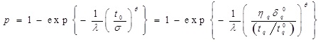
In this section, we provide a brief summary about the odds exponential log logistic distribution. The OELLD was introduced and studied quite extensively by Rosaiah et al. [1]. The probability density function (pdf) and cumulative distribution function (cdf) of OELLD respectively are given as follows:
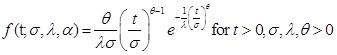 |
(1) |
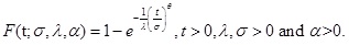 |
(2) |
where, λ, σ are the scale parameters and θ respectively shape parameters.
The 100q-th quantile of the OELLD is given as:
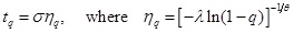 |
(3) |
Hence, for the fixed values of λ = λ 0 and θ = θ 0 , the quantile tq given in Equation (3) is the function of scale parameter σ = σ 0, that is
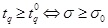 , where
 |
(4) |
Note that σ 0 also depends on λ 0 = θ 0, to build up acceptance sampling plans for the OELLD ascertain tq ≥ tq 0, equivalently that σ exceeds σ 0.
3. THE ACCEPTANCE SAMPLING PLAN
In this paper, we obtain the minimum sample size necessary to ensure a percentile life when the life test is terminated at a pre-assigned time t 0q and when the observed number of failures does not exceed a given acceptance number c. The decision procedure is to accept a lot only if the specified percentile of lifetime is established with a pre-assigned high probability α, which provides protection to the consumer. The life test experiment gets terminated at the time at which (c + 1)th failure is observed or at quantile time tq, whichever is earlier. Acceptance sampling plan based on truncated life tests for the OELLD using average life was discussed by Rosaiah et al. [1].
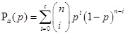
The probability of accepting lot based on the number of failures from all groups under a truncated life test at the test time schedule is given by
 |
(5) |
Where n is the sample size, c is the acceptance number, and p is the probability of getting a failure within the life test schedule t 0,. If the product lifetime follows an OELLD, then p = F(t 0). Usually, it would be convenient to determine the experiment termination time t 0 as t 0 = δq 0 tq 0 for a constant δq 0 and the targeted 100q-th lifetime percentile, t q 0. Suppose tq is the true 100q-th lifetime percentile. Then, p can be rewritten as
 |
(6) |
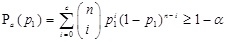
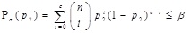
In order to find the design parameters of the proposed acceptance sampling plan, we prefer the approach based on two points on the OC curve by considering the producer’s and consumer’s risks. In our approach, the quality level is measured through the ratio of its percentile lifetime to the lifetime, tq/tq0. These percentile ratios are very helpful for the producer to enhance the quality of products. From the producer’s perspective, the probability of lot acceptance should be at least 1 - α at the acceptable reliability level (ARL), p1. So the producer demands that a lot should be accepted at various levels, say tq/tq0 = 2, 4, 6, 8, 10 in Equation (5). On the other hand, from the consumer’s viewpoint, the lot rejection probability should be at most β at the lot tolerance reliability level (LTRL), p2. In this way, the consumer considers that a lot should be rejected when tq/tq0 = 1. From Equation (5), we have
 |
(7) |
 |
(8) |
where p1 and p2 are given by
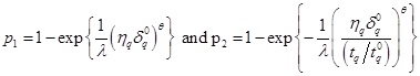 |
(9) |
The plan parametric quantities for distinct values of parameters λ are θ constructed. Given the producer’s risk α = 0.5 and termination time schedule t 0 = δq 0tq 0 with δq 0 = 1.0,1.5,2.5,2.0,3.0, the two parameters of the proposed sampling plan under the truncated life test at the pre-specified time, t 0, with λ = 2 and θ = 0.1,1.0,2.0 are obtained according to the consumer’s confidence levels β = 0.25,0.10,0.05,0.01 for 50th percentile and the operating characteristic values are also calculated and the results are presented in Tables 1-3. The plan parameters are presented in Tables 1-3 for λ = 2 and θ = 1.0,1.5,2.0 with 50th percentiles, whereas Table 4 shows the plan parameters for  and
and  are the MLE’s from the data given in Subsection 4.2 at 50th percentile. We noticed from Tables 1-4 that the percentile ratio increases, the sample size n decreases for all the cases. The sampling plans for OELLD were developed by Rosaiah et al. [1].
4. DESCRIPTION OF THE PROPOSED METHODOLOGY AND REAL DATA EXAMPLE
4.1. Description of the Proposed Plan
Assume that the producer wants to implement a single sampling plan for assuring that the 50th percentile life of the products under inspection is at least 1000 hours when = β 0.10 at the percentile ratio tq/tq0. He wants to run this experiment for 1000 hours. From the past data, if it is observed that the lifetime of the product follows OELLD with λ = 2 and θ = 2. The optimal plan from Table 3 for specified requirements such as β = 0.10, λ = 2, θ = 2, tq/tq0 = 2 and δq = 1.0 is obtained as n = 17 and c = 5 with the acceptance probability is 0.9587. To the best our knowledge, most of the life testing with single sampling plans for various life time distributions available in the literature is based on one point on the OC curve approach for assuring mean or percentile life time (except Balamurali et al. [17]). But in this study, we have designed sampling plans based on two-points on the OC curve approach for assuring percentile life time of the products under OELLD.
4.2. Real Data Example
In this section, we present the application of the proposed OELLD distribution considered by Lemonte [18] for a real data set to illustrate its potentiality. The following real data set corresponds to an uncensored data set from Nichols and Padgett [19] on breaking stress of carbon fibres (in Gba):
| 0.39, 0.81, 0.85, 0.98, 1.08, 1.12, 1.17, 1.18, 1.22, 1.25, 1.36, 1.41, 1.47, 1.57, 1.57, 1.59, 1.59, 1.61, 1.61, 1.69, 1.69, 1.71, 1.73, 1.80, 1.84, 1.84, 1.87, 1.89, 1.92, 2.00, 2.03, 2.03, 2.05, 2.12, 2.17, 2.17, 2.17, 2.35, 2.38, 2.41, 2.43, 2.48, 2.48, 2.50, 2.53, 2.55, 2.55, 2.56, 2.59, 2.67, 2.73, 2.74, 2.76, 2.77, 2.79, 2.81, 2.81, 2.82, 2.83, 2.85, 2.87, 2.88, 2.93, 2.95, 2.96, 2.97, 2.97, 3.09, 3.11, 3.11, 3.15, 3.15, 3.19, 3.19, 3.22, 3.22, 3.27, 3.28, 3.31, 3.31, 3.33, 3.39, 3.39, 3.51, 3.56, 3.60, 3.65, 3.68, 3.68, 3.68, 3.70, 3.75, 4.20, 4.38, 4.42, 4.70, 4.90, 4.91, 5.08, 5.56. |
The goodness of fit for our model by plotting the superimposed for the data shows that the OELLD is a good fit in the Figure and also goodness of fit is emphasized with Q-Q plot, displayed in the Fig. (1). The maximum likelihood estimates of the two-parameters of OELLD for the breaking stress of carbon fibres are and and the Kolmogorov-Smirnov test we found that the maximum distance between the data and the fitted of the OELLD is 0.0604 with p-value is 0.8582. Therefore, the three-parameter OELLD provides reasonable fit for the breaking stress of carbon fibres.
 |
Fig. (1). Estimated density and Q-Q plot for OELLD. |
Suppose that it is desired to develop the single acceptance sampling plan to satisfy that the 50th percentile lifetime is greater than breaking stress of carbon fibres 0.35 through the experiment to be completed by breaking stress of carbon fibres/measurement 0.35. Let us fix that the consumer's risk is at 25% when the true 50th percentile is breaking stress of carbon fibres 0.35 and the producer's risk is 5% when the true 50th percentile is breaking stress of carbon fibres 0.70. Since and , the consumer's risk is 25%, δq 0 = 1.0 and tq/tq 0 = 2, the minimum sample size and acceptance number given by n = 7 and c = 2 from Table 4. Thus the design can be implemented as follows. Select a sample of 7 runoff amounts, we will accept the lot when no more than two failures occurs before breaking stress of carbon fibres 0.70. According to this plan, the breaking stress of carbon fibres could have been accepted because there is only one failure before the termination time, breaking stress of carbon fibres 0.70.
CONCLUSION
In this article, we developed the single acceptance sampling plans based on the OELLD percentiles, when the life test is truncated at a pre-fixed time. To ensure that the life quality of products exceeds a specified one in terms of the percentile lifetime, the acceptance sampling plans based on percentiles can be used. We have designed sampling plans based on two-points on the OC curve approach for assuring percentile lifetime of the products. Some tables are provided for practical use in industry and also proposed plan illustrated with real data set. We fitted the proposed OELLD curve for the above data which is shown in Fig. (1).
CONFLICT OF INTEREST
The authors confirm that this article content has no conflict of interest.
ACKNOWLEDGEMENTS
Declared none.