
RESEARCH ARTICLE
Consistency of the Semi-parametric MLE under the Cox Model with Right-Censored Data
Qiqing Yu1, *
Article Information

Identifiers and Pagination:
Year: 2020Volume: 10
First Page: 21
Last Page: 27
Publisher Id: TOSPJ-10-21
DOI: 10.2174/2666148902010010021
Article History:
Received Date: 14/05/2020Revision Received Date: 14/08/2020
Acceptance Date: 19/08/2020
Electronic publication date: 23/10/2020
Collection year: 2020
open-access license: This is an open access article distributed under the terms of the Creative Commons Attribution 4.0 International Public License (CC-BY 4.0), a copy of which is available at: https://creativecommons.org/licenses/by/4.0/legalcode. This license permits unrestricted use, distribution, and reproduction in any medium, provided the original author and source are credited.
Abstract
Objective:
We studied the consistency of the semi-parametric maximum likelihood estimator (SMLE) under the Cox regression model with right-censored (RC) data.
Methods:
Consistency proofs of the MLE are often based on the Shannon-Kolmogorov inequality, which requires finite E(lnL), where L is the likelihood function.
Results:
The results of this study show that one property of the semi-parametric MLE (SMLE) is established.
Conclusion:
Under the Cox model with RC data, E(lnL) may not exist. We used the Kullback-Leibler information inequality in our proof.
1. INTRODUCTION
We studied the consistency of the semi-parametric maximum likelihood estimator (SMLE) under the Cox model with right-censored (RC) data.
Let Y be a random survival time, X a p-dimensional random covariate. Conditional on X = x, Y satisfies the Cox model if its hazard function satisfies
 |
(1.1) |
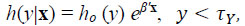
where ho is the baseline hazard function, i.e., ho (y) = fo (y) /So (y-), fo is a density function, So (y) = S(y|0)  P (Y > y |X = 0), Fo = 1 - So, τY = sup{t:SY(t) > 0}, h(y|x) =
  , S(·|·) f(·|·) orF(·|·)) is the conditional survival function (density function (df) or cumulative distribution function (cdf)) of Y given X = x. The restriction y<τY is not in the original definition of the PH model, but is necessary if So is discontinuous at τY (see Remark 1 [1])
2. METHODS
In this paper, we shall make use of the assumptions as follows:
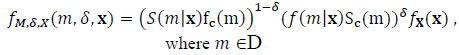
AS1. Suppose that C is a random variable with the df fC (t) and the survival function SC (t), X takes at least p +1 values, say 0 , x1, ..., xp, where x1, ..., xp are linearly independent, (Y,X) and C are independent. Let (Y1,X1,C1), ..., (Yn,Xn,Cn) be i.i.d. random vectors from (Y,X,C). M = min(Y,C) and δ = 1(Y ≤ C), where 1(A) is the indicator function of the event A. Let (M1, δ1X1), ..., (Mn, δn, Xn) be i.i.d. RC observations from (M, δ, X) with the df are as follows:
 |
(1.2) |
 |
and S(t|x) is a function of (So, β) (see Eq. (1.1)), but not fx and fC (the df’s of X and C).
Due to (AS1) and Eq. (1.2), the generalized likelihood function can be written as:
 |
(1.3) |
which coincides with the standard form of the generalized likelihood [2]. Eq. (1.3) is identical to the next expression:
 |
(1.4) |
where ηn = min{|Mi {1,2, ..., n}}. This form allows So to be arbitrary (discrete or continuous, or others), thus is more convenient in the later proofs. If Y is continuous then S(t|x) = (S(t|0))exp(X'β) = (So (t))exp(X'β), but
 |
(1.5) |
If Y is discrete then S(t|x) = ∏s≤t(1 - h(s|x)) = ∏s≤t(1 - h0 (s)eX'β) If Y has a mixture distribution, then S(t|x)= p (S01(t))exp(X'β) + (1 - p) ∏s≤t(1 - h02(s)eX'β where p (0,1), h01 and h02 are two hazard functions. h0 (t) = ph01 + (1 - p)h02 and S0 (t) = pS01 + (1 - p)S02
The SMLE of (So, β) maximizes L (S, b) overall possible survival function S and bRp, denoted by ( ). The SMLE of S(t|x) is denoted by
  (t|x), which is a function of (). The computation issue of the SMLE under the Cox model has been studied, but its consistency has not been established under the model [3]. Their simulation results suggest that the SMLE is more efficient than the partial likelihood estimator under the Cox model.
The partial likelihood estimator is a common estimator under the Cox model, which maximizes the partial likelihood: 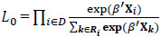 , where D is the collection of indices of the exact observations and Ri is the risk set {j: Mj ≥ Yj}. The asymptotic properties of the estimator are well understood [4].
The consistency of the SMLE under the continuous Cox model with interval-censored (IC) data has been established, making use of the following result [5]:
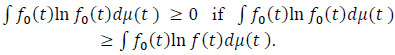
The Shannon-Kolmogorov (S-K) inequality. Let fo and f be two densities with respect to (w.r.t.) a measure μ and ∫ f0 (t)ln f0 (t)dμ(t) is finite. Then, ∫ f0 (t)ln f0 (t)dμ(t) ≥ ∫ f0 (t)ln f (t)dμ(t), with equality iff f = fo a.e. w.r.t. μ.
Under the Cox model with IC data, the S-K inequality becomes E (lnL(So, β))  (S, b), where L(Rp. Their approach cannot be extended to the Cox model with RC data as the key assumption (in the S-K inequality) [3].
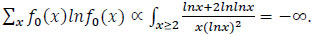
That is, finite E (lnL (So, β)), may not hold. Indeed, if Y has a df 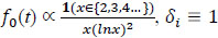 and β = 0, then L
A related inequality is as follows.
The Kullback-Leibler (K-L) information inequality. Let fo and f be two densities w.r.t. a measure μ. Then ∫ f0 (t)ln (f0 /f)(t)dμ(t) ≥ 0, with equality iff f = foa.e. w.r.t. μ.
The K-L inequality says that ∫ f0 (t)ln (f0 /f)(t)dμ(t) exists, though it maybe
 |
In this note, we show that the SMLE under the Cox model is consistent, making use of the Kullback-Leibler information inequality [6]
2. The Main Results. Notice that under the assumption that ho exists, So, fo, Fo and ho are equivalent, in the sense that given one of them, the other 3 functions can be derived. Thus, the Cox model is applicable only to the distributions that the density functions exist, that is, Y is either continuous, or discrete, or the mixture of the previous two. Since the expression of S(t|x) varies in these three cases, for simplicity, we only prove the consistency of the SMLE under the Cox model in the first two cases.
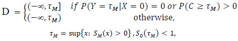
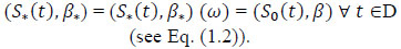
Theorem 1. Under the Cox model with RC data, if Y is either continuous or discrete, and ifSo (τM) <1, then the SMLE ( ) is consistent t D (see Eq. (1.2)).
The proof of Theorem 1 makes use of a modified K-L inequality. K-L inequality requires that f0 and f are both densities w.r.t. the measure μ. That is ∫ f(t)dμ(t = 1. However, in our case, we encounter the case that ∫ f(t)dμ(t) [0,1].
Lemma 1 (the modified K-L inequality). If fi ≥ 0, μ1 is a measure, ∫ f1(t)dμ1(t = 1 and ∫ f2(t)dμ1(t ≤ 1, then ∫ f1(t)ln  dμ1(t) ≥ 0, with equality iff f1 = f2 a.e. w.r.t. μ1.
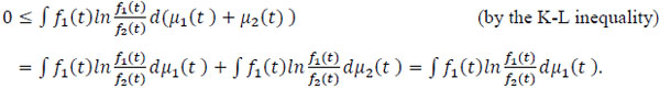
Proof. In view of the K-L inequality, it suffices to prove the inequality ∫ f1(t)ln dμ1(t) ≥ 0 under the additional assumptions that ∫ f2(t)dμ1(t < 1, ∫ f1(t)dμ2(t = 0 and ∫ f2(t)dμ(t < 1, where μ2 is a measure and μ = μ1 + μ2 Since ∫ f2(t)dμ(t) = 1, f1 and f2 are df's w.r.t. μ.
 |
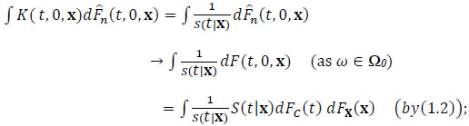
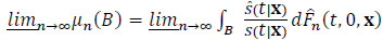
Proof of Theorem 1. Let Ω0 be the subset of the sample space Ω such that the empirical distribution function (edf)  , (t, s, x) based on (Mi, δi, Xi) converges to F(t,s,x), the cdf of (M, δ, X). It is well-known that P(Ω0,) =1. Notice that the SMLE () is a function of (ω, n), say (o,n (t)(ω),
  o,n (tn)(ω) , where ω Ω and n is the sample size. Hereafter, fix an ω Ω0 , since (=n(ω)) is a sequence of vectors in Rp, there is a convergent subsequence with the limit β*, where the components of β* can be o, there exists a further subsequence which is convergent. Without loss of generality (WLOG), we assume that o → S* and → β*. Of course, (β*, S*) depends on ω( Ω0 ). We prove in Theorem 2 for the discrete case and in Theorem 3 for the continuous case that:
 |
(2.1) |
Since ω can be arbitrary in Ω0 and P(Ω0 ) = 1, the SMLE is consistent.
Before we prove Theorems 2 and 3, we present a preliminary result.
Lemma 2 (Proposition 17 in Royden (1968), page 231). Suppose thatμn is a sequence of measures on the measurable space (J,  ) such that μn(B) μ(B),B, gn and fn are non-negative measurable functions, and
  (fn, gn)(x) = (f, g)(x) Then,
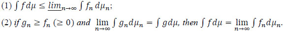
Corollary 1. Suppose that μn is a sequence of measures on the measurable space (J , B) such that μn (B) → μ (B), B, f andfn (n ≥ 1) are integrable functions that are bounded below andf(x)n→∞ = lim fn(x). Then ∫ f dμ ≤ limn→∞ ∫ fn dμn.
Proof. Let k = infn infxfn(x). If k ≥ 0 then the corollary follows from Lemma 2. Otherwise, let fn-(x) = 0 Λ fn(x), fn+(x) = 0 v fn(x), f-(x) = 0 Λ f(x) and f +(x) = 0 v f(x). Then, fn+ → f + and fn- → f - point wisely, as, fn → f
limn→∞ ∫ fn dμn = limn→∞ ∫ (fn+ + fn-)dμn = limn→∞ [∫ fn+ dμn + fn- dμn] ≥ ∫ limn→∞fn+ dμ + ∫ limn→∞fn- dμ (by Lemma2, as fn+ (x) is nonnegative and |f- (x)| ≤ k) = ∫ f + dμ + ∫ f- dμ = ∫ (f + + f-)dμ = ∫ f dμ.
Theorem 2. Under the discrete Cox model with RC data, Eq. (2.1) holds.
Proof. For the given ω Ω0 and (S*, β*) in the proof of Theorem 1, as assumed, () (ω) → (S*, β*). Defining h*(t) =  and h*(t|x) = h*(t)eβ*'x (for S*(t -) > 0) yeilds S*(t|x) and f*(t|x), which are continuous functions of S* and β*. Consequently, (·|·) → S*(·|·).
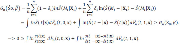
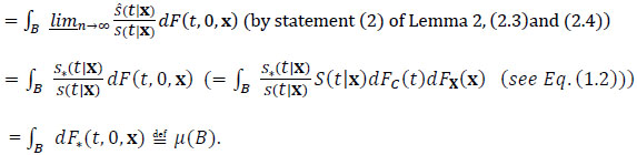
Let Gn(S0 , β) = lnL(S0 , β)/n (see Eq.(1.3)). Then, the SMLE () satisfies
 |
(2.2) |
 |
. |
where B is a measurable set in Rp+1. To apply Lemma 2,
 |
(2.3) |
 |
(2.4) |
 |
(2.5) |
 |
(2.6) |
 |
(2.7) |
 |
(2.8) |
 |
 |
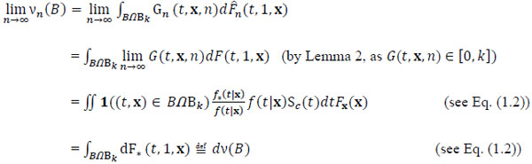
(2.9) |
 and vn converges set wisely to a finite measure v (see (2.9)), by a similar argument as in (2.4), (2.6), (2.7) and (2.8), we have:
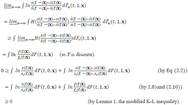 |
(2.10) |
Thus, ∫ ln dF(t, 0, x) + ∫ ln
 dF(t, 1, x). Hence, (S0 (t),β) = (S*(t),β)tD by the 2nd statement of the K-L inequality.
Theorem 3.Under the Cox model with RC data, if Y is continuous then Eq. (2.1) holds.
Proof. For the given ωΩ0 and (S*,β*) in the proof of Theorem 1, as well as (ω) and (t|x)(ω), we have S*(t|x) = (S*(t))exp(β*'x). By a similar argument as in proving Eq. (2.8), we can show:
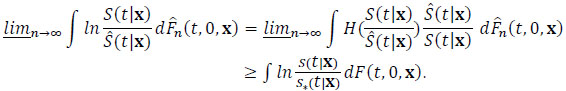 |
(2.11) |
In view of Eq. (1.4) due to Y is continuous, we denote:
 |
(2.12) |
 |
(2.13) |
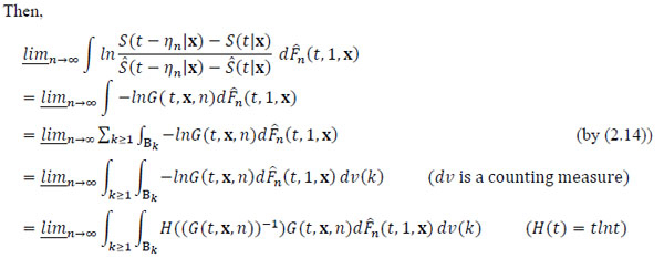
as S* is a monotone function, S*' exists a.e., and so do S*'(t|x) and F*'(t|x). We have
 |
(2.14) |
The reason is as follows. For each (t, x) such that F'(t|x) > 0 and Eq. (2.13) holds,
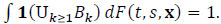
F*'(t|x) /F'(t|x) (=f*(t|x) /f (t|x)) is finite. Then, there exists no such that G(t, x, n) < 1 + F*'(t|x) /F'(t|x) for n ≥ no . On the other hand, G(t, x, n) is finite for n =1, ..., no . Thus, G(t, x, n) < k for some k. Since Eq. (2.1) holds a.e. and ∫ 1dF(t, s, x) = 1, Eq. (2.14) holds.
We shall prove in Lemma 3 that
 |
(2.15) |
 |
. |
 |
(2.16) |
 |
. |
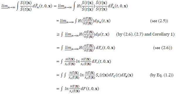
3. RESULTS
The last inequality further implies that ∫lnd F(t,0,x) + ∫ln d F(t,1,x) = 0. Thus, (S0 (t),β) = (S*(t),β*) t D by the 2nd statement of the K-L inequality and by the assumption ASI.
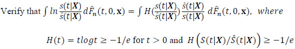
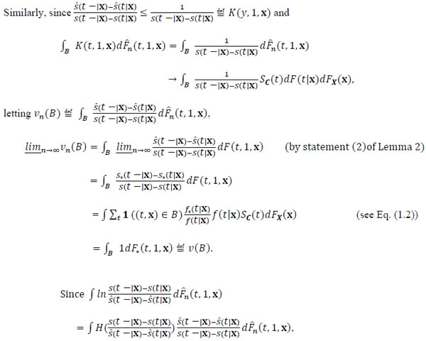
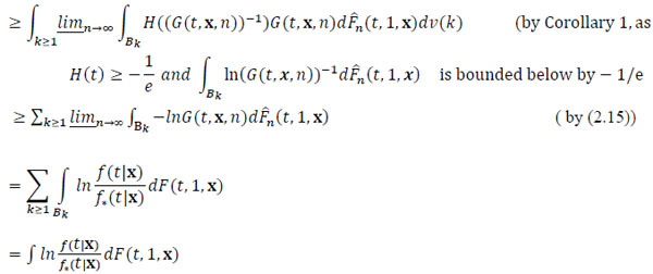
Lemma 3. Inequality (2.15) holds.
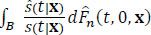
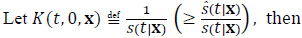
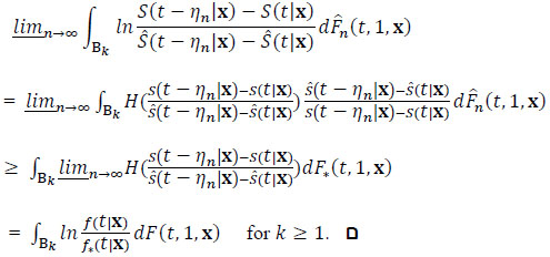
Proof. Let k ≥ 1 and  , where B is a measurable set and
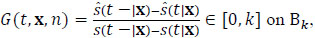
 |
. |
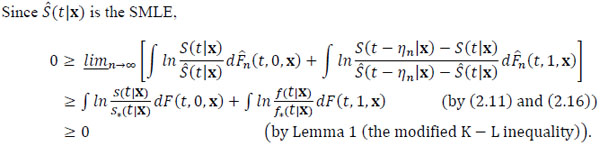
CONCLUSION
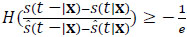
Since H((S (t-ηn|x) - (S (t|x))/(( (t-ηn|x) - ( (t|x))) ≥ - 1/e and vn converges set wisely to a finite measure v by a similar argument as in (2.4), (2.6), (2.7) and (2.8), we can show that:
 |
. |
CONSENT FOR PUBLICATION
Not applicable.
AVAILABILITY OF DATA AND MATERIALS
Not applicable.
FUNDING
None.
CONFLICT OF INTEREST
The author declare no conflict of interest, financial or otherwise.
ACKNOWLEDGEMENTS
The author would like to thank the editor and two referees for their invaluable comments.