
RESEARCH ARTICLE
Asymptotic Relative Efficiencies of the Score and Robust Tests in Genetic Association Studies
Ao Yuan1, *, Ruzong Fan1, Jinfeng Xu2, Yuan Xue3, Qizhai Li4
Article Information

Identifiers and Pagination:
Year: 2018Volume: 9
First Page: 26
Last Page: 41
Publisher Id: TOSPJ-9-26
DOI: 10.2174/1876527001809010026
Article History:
Received Date: 7/3/2018Revision Received Date: 23/7/2018
Acceptance Date: 2/10/2018
Electronic publication date: 28/12/2018
Collection year: 2018
open-access license: This is an open access article distributed under the terms of the Creative Commons Attribution 4.0 International Public License (CC-BY 4.0), a copy of which is available at: https://creativecommons.org/licenses/by/4.0/legalcode. This license permits unrestricted use, distribution, and reproduction in any medium, provided the original author and source are credited.
Abstract
Introduction:
The score statistic Z(θ) and the maximin efficient robust test statistic ZMERT are commonly used in genetic association study, but according to our knowledge there is no formal comparison of them.
Methods:
In this report, we compare the asymptotic behavior of Z(θ) and ZMERT, by computing their Asymptotic Relative Efficiencies (AREs) relative to each other. Four commonly used ARE measures, the Pitman ARE, Chernoff ARE, Hodges-Lehmann ARE and the Bahadur ARE are considered. Some modifications of these methods are made to simplify the computations. We found that the Chernoff, Hodges-Lehmann and Bahadur AREs are suitable for our setting.
Results and Conclusion:
Based on our study, the efficiencies of the two test statistic varies for different criterion used, and for different parameter values under the same criterion, so each test has its advantages and dis-advantages according to the criterion used and the parameters involved, which are described in the context. Numerical examples are given to illustrate the use of the two statistics in genetic association study.
1. INTRODUCTION
In genetic association studies, several test statistics are often used, including the score test Z(θ) and the maximin efficient robust test statistic ZMERT. Although numerical behavior of the two tests are reported in various genetic association studies based on simulations, to our knowledge, a formal theoretical comparison of the two tests hasn’t been seen in the literature. It is of meaning to compare their asymptotic performances. Although for likelihood ratio based test statistic for testing hypothesis of simple null versus simple alternative, there is a uniformly most powerful test under some regularity conditions. However, most test statistics are not constructed directly from likelihood ratio, the hypothesis are composite, and there is generally no such optimal test. Therefore, the classical method to compare any two test statistics is to evaluate the Asymptotic Relative Efficiency (ARE) between them.
The ARE is a well studied area, with vast literatures and numerous different definitions. But often the computation of ARE is very difficult in the general case, some of the classical methods for ARE require that the test statistics have some standard forms, such as they have the same asymptotic distribution, or have the forms of i.i.d. summations. However, in practice, such as in genetic association studies, some test statistics do not have these forms. Sitlani and McKnight [1] studied AREs for the trend test under different models and stratifications. In this communication, wecompare the asymptotic behavior of two commonly used test statistics the score statistic Z(θ) and the maximin efficient robust test statistic ZMERT, arise in case-control genetic association study, as given in Zheng, Li and Yuan [2], hereafter ZLY, by evaluate their AREs relative to each other. Four commonly used ARE measures, the Pitman ARE, Chernoff ARE, Hodges-Lehmann ARE and the Bahadur ARE are considered. Pitman’s ARE does not apply directly. We found the Chernoff, Hodges-Lehmann and the Bahadur AREs are suitable for our setting. Some modifications of these methods are made to simplify the computations.
Existing studies on ARE are mainly focused on two categories. One is to compare efficiencies of estimators of the same parameter; the other is to compare test statistics of the same hypothesis, in which the test statistics may not estimate the same parameter. The latter study can be under the assumption that the test statistics in comparison are asymptotic normality. In this case, the ARE’s can often be easily computed. There are also methods for compare ARE of different test statistics in general, in which different test statistics of the same hypothesis may have different asymptotic distributions. In this general case, Pitman, Bahadure and Hodges-Lehmann proposed different ways to compute the ARE, and it is often difficult. Although, when the test statistics have the same asymptotic distribution, the ARE can be computed easily. We also give a simple definition of ARE, so that it can be computed in the case of different asymptotic distributions, as long as the asymptotic distributions of the test statistics are known.
In Section 2, we describe the background of the genetic association study problem and a brief review of the classical definitions of ARE. In Section 3 we compare the ARE of the test statistics arose from our genetic association study. We found that he performances, or the efficiencies of the two test statistic varies for different criterion used, and for different parameter values under the same criterion, which described in the context. Section 4 gives brief numerical examples in simulation and application of the two tests in genetic association study, from our previous study, to illustration their usage.
2. BACKGROUND
Denote the log-likelihood function as,
 where Yi is the outcome,
 R2 are the parameters of interest,
 is a vector of parameters (m ≥ 0) for the covariate Xi = (x1,....,xim)T, and n is the sample size. The goal is to test the null hypothesis
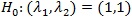 against the alternative H1 (λ1, λ2)
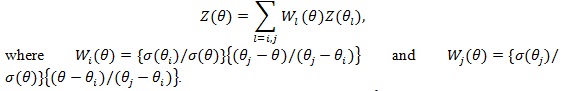
 \ {(1, 1)}, where
has two edges with known slopes θ 0 and θ1, and the null point (1, 1) is on the boundary of
. We assume - ∞ < θ 0 < θ1 <∞ and the endpoints θ 0 and θ1 satisfy some constraints as specified in ZLY. If θ1 = ∞ which corresponds to a vertical edge, we can switch λ1 and λ2 and define new (θ1, θ2) so - ∞ < θ 0 < θ1 <∞ is satisfied by the new (θ1, θ2). For example, we can write λ1 = 1 + (λ2 - 1)/ λ1* (λ2-1) and λ1 = 1 + (λ2 - 1)/ θ 0 = 1 + θ 0* (λ2 - 1) where - ∞ < θ 0 < θ1 <∞.
\ {(1, 1)}, where
has two edges with known slopes θ 0 and θ1, and the null point (1, 1) is on the boundary of
. We assume - ∞ < θ 0 < θ1 <∞ and the endpoints θ 0 and θ1 satisfy some constraints as specified in ZLY. If θ1 = ∞ which corresponds to a vertical edge, we can switch λ1 and λ2 and define new (θ1, θ2) so - ∞ < θ 0 < θ1 <∞ is satisfied by the new (θ1, θ2). For example, we can write λ1 = 1 + (λ2 - 1)/ λ1* (λ2-1) and λ1 = 1 + (λ2 - 1)/ θ 0 = 1 + θ 0* (λ2 - 1) where - ∞ < θ 0 < θ1 <∞.
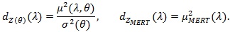
Assume θ 0 and θ1 are known from the problem of interest and/or scientific knowledge. Given λ1 = λ ≥ 1, λ2 can be written as
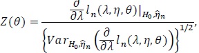
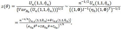
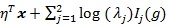
 . We treat η as a nuisance parameter not estimable under H 0 λ = 1, but it is estimable under 0. Then the log-likelihood becomes. ln (λ, η, θ) The score test statistic H 0 λ = 1 for is given by;
 |
(1) |
where
 is the MLE of η under H 0. It would be difficult to deal with ln (λ, η, θ) because θ in Z (θ) is implicitly expressed.
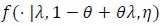
So we work with ln (λ,1 - θ + θλ, η), where θ is explicitly expressed. It is convenient to view ln (λ, η, θ) as a tri-variate function with variables x1 = λ, x2 = 1 - θ + θλ and x3 = η. Denote ln,u = ∂ln/ ∂xu for, u = 1,2,3, ln, uv = ∂2ln/∂xu∂xv for u = 1,2 and, v = 1.2.3, and ln.33 = ∂2ln/∂x3∂xT3. Assume
 and v = 3. Denote Lvu (η) = EHnllvu (1.1, η).
Suppose we have a family of asymptotically normally distributed tests
 , where
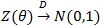 under H1 λ = 1 for a given
 , which determines the data-generating model under H 0: λ = 1. When
 is the true value Z(θ()), is asymptotically most powerful (optimal). In this case, θ(1) ≠ θ(0) when is used, the Pitman ARE of Z(θ(1)) relative to Z(θ(1)) is given by (Gastwirth [3, 4])
 |
(2) |
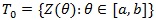
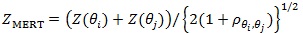
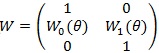
where is the asymptotic null correlation coefficient between and. Let be a set of all convex linear combinations of. A simple robust test derived under efficiency robust theory (Gastwirth [3, 4]; Birnbaum and Laska [5],) is the maximin efficient robust test (MERT), denoted as. When, is given by;
 |
(3) |
When T 0 has more than two members, generally exists and is unique (Gastwirth [3]), but its computation needs quadratic programming methods (Rosen [6]). However, when there is an extreme pair (Z(θi), Z(θ i)) in T 0i.e. pθi, θi =
 is MERT for if and only if (Gastwirth [7]).
 |
and thus
 |
(4) |
That is, the MERT reaches the maximin ARE due to model uncertainty. The MERT was first derived for linear rank tests for the two-sample problem (Gastwirth [3]; Birnbaum and Laska [5],) and later extended to a family of asymptotically normally distributed tests (Gastwirth [4]).
The Z (θ) statistic has the following property (ZLY): Let.
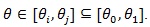 Then where and.
 |
Let
 be the MLE of η under H 0, and
 be that of (η, λ) under H1. For given θ, the X2 likelihood ratio test statistic is
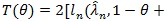
 . For fixed θ, the number of parameters under H1 is just 1 more than that under H 0, so by Wilk’s theorem, under H 0,
 |
the chi-squared distribution with one degree of freedom. The likelihood ratio test is also widely used in genetic association studies, its properties, including its ARE is well studied in the literature, so we will not investigate it here.
Let the MLE
 here 0 presents a vector of 0’s. Let η 0 be the true value (unknown) of η under either H 0 or H1, we define the score function as;
 |
and the test statistic for H 0 as;
 |
(5) |
where “~” means asymptotically equivalent, in the above
 is replaced by
 it is approximated by n-1ln, vu (1.1, η).
Denote
 . For a vector v (v1, v2, v3)T, denote
 . be the true density of the data y. The null model f (1, 1, η) is and the alternative model is
 . The following notation is also used under H1. For fixed, (λ, θ) let;
 |
(6) |
Under H1, the empirical version of η 0 is just
 . We denote the Fisher information and its inverse in the blocked forms as;
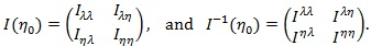 |
Let


by
 is replaced by
 Note that with
 defined in the above,

Below we give a brief review of the notions of ARE for test statistics in the general case, more detailed account can be found in Serfling (1980) [8] and Nikitin (2011) [9].
The calculation of the existing of versions of ARE is generally not easy, as in the examples (Serfling, 1980 [8]; Nikitin, 1995 [10]; van der Varrt, 1998 [11]). We only point out that the Pitman ARE is based on the central limit theorem for test statistics, that the Bahadur ARE requires the large deviation asymptotics of test statistics under the null-hypothesis, while the Hodges-Lehmann ARE is connected with large deviation asymptotics under the alternative. Each type of ARE has its own advantage and dis-advantage, and the different notions of ARE are not always give consistent conclusion.
If the condition of asymptotic normality (or common asymptotic distribution) fails, considerable difficulties will arise in calculating the Pitman ARE as it may not at all exist or may depend on α and β. Usually one considers limiting Pitman ARE as α → 0 Wieand (1976) [12] established the correspondence between this kind of ARE and the limiting approximate Bahadur efficiency which is easy to compute.
The Bahadur (1960) [13] ARE is to fix the power of tests and compare the exponential rate of decrease of their sizes for the increasing number of observations and fixed alternative. Its computation is always non-trivial, and heavily depends on advancements in large deviation theory, as in Dembo and Zeitouni (1998) [14] and Deuschel and Strook (1989) [15].
It is proved that under some regularity conditions the likelihood ratio statistic is asymptotically optimal in Bahadur sense (Bahadur, 1967 [16]; Arcones, 2005 [17]). Often the Bahadur ARE is difficult to compute for any alternative but it is possible to calculate the limit of Bahadur ARE as θ approaches the null-hypothesis, to obtain the local Bahadur efficiency.
The Hodges-Lehmann ARE is, in contrast to Bahadur efficiency, it fixes the level of tests and compares the exponential rate of decrease of their type-II errors for the increasing number of observations and fixed alternative. The computation of Hodges-Lehmann ARE is also difficult as it requires large deviation asymptotics of test statistics under the alternative.
The drawback of Hodges-Lehmann efficiency is that most two-sided tests like Kolmogorov and Cramer-von Mises tests are all asymptotically optimal, and hence one cannot discriminate among them. On the other hand, under some regularity conditions the one-sided tests, such as linear rank tests can be compared, and their Hodges-Lehmann efficiency coincides locally with Bahadur efficiency (Nikitin, 1995 [10]).
The Chernoff ARE is to minimize, asymptotically, a linear combination of type I and type II errors, it does not depend on the nominal level nor the power. But it basically only applies to test statistics of the form of i.i.d. summation.
The local ARE is much easier to compute than the previous ones, but it only applies to test statistics which are asymptotical normal with rate
 . We will see that some test statistics used in genetic association studies do not satisfy this condition.
Besides the four commonly used AREs for hypothesis tests described above, there are some other interesting methods. Hoeffding’s (1965) ARE [18], based on the work of Sanov (1957) [19], is theoretically appealing, but ony applies to multinomial data; Rubin and Sethurman ARE (1965) [20] is based on Bayes risk; others including Kallenberg ARE (1983) [21], and the Borovkov-Mogulskii ARE (1993) [22], etc.
3. ARE OF TWO TESTS IN GENETIC ASSOCIATION STUDIES
In this section, we investigate the uses of Pitman ARE, Chernoff ARE, Hodges-Lehmman ARE, and Bahadur ARE to the commonly used statistics in genetic association analysis. We focus on the statistics used in ZLY, Z(θ) and, ZMERTand refer the notations there. Although some other commonly used test statistics in genetic association studies, such as the likelihood ratio statistic (chi-squared statistic), we will not discuss them here, as most of them are well studied in the literatures.
Pitman ARE. Consider testing
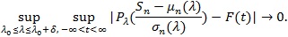
 Let Sn be a test statistic based on data of size n, with mean µn (λ) and standard deviation µn (λ). To use this method the following conditions are needed.
(P1). For some continuous strictly increasing distribution function F independent of λ, and some, δ > 0 as n → ∞,
 |
(P2). For
 , is k times differentiable, with µn(1) (λ 0) = ... =
(P3). For d(n) → ∞ some and some constant
(P4). For

Pitman appears as the first to introduce the notion of ARE for tests in his unpublished lectures, and the following result was stated in Noether’s works.
(Pitman, 1949 [23]; Noether, 1950 [24]). Assume (P1)-(P4), that αn = Pλ 0 (Sn >
 then
then
 , if and only if
 |
(7) |
(ii) Let S1,n and S2,n each satisfy (P1)-(P4) with the common F, K, n1 and n2 be the sample size required for S1,n and S2,n to have the same asymptotic power 1 - β, then
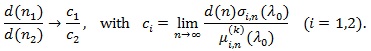 |
Thus, if d(n) = nq (q > 0), then the Pitman ARE is given by;
 .
.
 |
and Pitman ARE is then;
 |
(8) |
Let l (λ 0) be the Fisher information at λ 0. Under some additional conditions, Rao (1963) [25] proved that
 |
Any test statistic Sn achieves the equality in the above is called Pitman efficient.
Under suitable conditions, Pitman ARE can be expressed in terms of correlation coefficient between the two test statistics in their standardized form, as given below.
(P5)
 are asymptotic joint normal uniformly in a neighborhood of λ0.
Denote p(λ)the asymptotic correlation coefficient between them under, and and be the distribution and density function of. The following result is true.
(van Eden, 1963 [26]). Assume that S1,n and S2,n satisfy (P1)-(P5) in their standardized form with
 , and that p(λn) → p(λ λn): = p as λn → λ 0 Then;
(i) For 0 ≤ λ ≤ 1, tests of the form
 satisfy (P1)-(P5), and the “best” Syn which maximizes
 is the one with;
 |
and
 |
(9) |
(ii) If S1n is the best test satisfying (P1)-(P5), then;
 |
(10) |
In the typical case, Sn is an i.i.d. summation (upto scale), then µn(λ) = nµ(λ)

Note
 does not (α, β) depend on , thus if
 or, C1 > C2 then {S1n} is better than {S2n} for all (α, β).
Pitman ARE given by (3) or (4) are easy to use. However, they require the two comparing test statistics have the same asymptotic distribution (after standardization), (4) require further that they are jointly asymptotic normal. In practice, these conditions some times cannot be satisfied. For example the chi-squared test Z (θ 0) and have different asymptotic distributions. Below we give a generalized version of (3) to the case the two comparing test statistics not necessarily have the same asymptotic distribution (after standardization). Similar generalizations may have already exist in the literature, we still state our version to see what form it has in this case. Let Fi be the asymptotic distribution of
 We have;
Assume (P1)-(P4) for Sin with µin, σin and Fi separately, but with the same K and nominal level α, n1 and n2 be the sample sizes required for S1n and N2n to have the same asymptotic power 1 - β(0 < β < 1 - α), then
 |
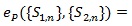
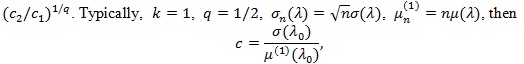
Thus for d(n) = nq (q > 0), we define the generalized Pitman ARE as;
 |
(11) |
In the typical case
 or 1/q = 2, and;
 |
Note, unlike the case of F1 = F2, in this case, Pitman’s ARE depends on the values of level α and power β , and comparison of two tests may not have consistent result.
Can we have the corresponding form of (10) in the case S1n and S2n have different asymptotic distribution? For this we checked the proof for (4), and find in this case, although in principle there is a relationship among the asymptotic correlation coefficient p between S1n and S2n , the asymptotic distributions’s, Fi's, and the level α and power β , but its mathematically intractable. Below we give its actual value.
Proposition 1.
 |
Remark: When some of the conditions (P1)-(P5) are not satisfied, ARE may not be characterized by correlation coefficient. For example, T1 = Z is an estimate of θ = 0 under H 0, and Z is symmetrically distributed around 0, so EHo (Z) = 0 and suppose VARHo (Z) = 1 . Let,
 is an estimate of
 can also be used to test H 0. However
 , but we cannot say that T2 is a ‘bad’ test statistic, and
 .
.
Chernoff ARE. This notion only considers test statistic of the form
 with the s i.i.d. with
 be the moment generating function of Y, and;
 |
Let
 and
and
 (assume µ 0 ≤ µ1),
 (i = 0,1),
 and
and
 is called the Chernoff index
 . be a linear combination of type I and type II errors evaluated at the critical value t, and Qn = infµ0 ≤ t ≤ µ,Qn (t) be the minimum of these errors for test statistic Sn. Chernoff (1952) [27] showed that Qn tends to 0 at exponential rate, (so the faster the rate, or the larger absolute value of logQn, the better the test statistic), and established.
 |
the result is independent of γ.
Let {S1,n} and {S2,n} both of the form of i.i.d. summation and have Chernoff indices p1 and p2 respectively, n1 and n2 be the corresponding sample sizes for which Q1,n, ~ Q2,n, the Chernoff ARE of {S1,n} relative to {S2,n} is defined and given by;
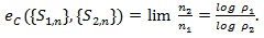 |
(12) |
For test statistic not in the form of i.i.d summation, its Chernoff index is difficult to compute. The following result sometimes is very helpful in this case, and give an upper bound of Chernoff index.
(Kallenberg, 1982 [28]) Let for some
 |
Then 
In the case of simple null vs simple alternative, Kallenberg (1982) [28] also gives an upper bound of the Chernoff index, and any test statistic achieves this bound is said to be Chernoff efficient. As this bound itself is not easy to compute, we won’t pursue it here, interested readers can check the mentioned paper or the book by Nikitin (1995) [10].
As another way to simplify the computation, we consider a modified version of this Chernoff index. Let S be the weak limit of Sn, be the distribution function of S, and Hn: λn + λn = n-1/2be a sequence of local alternatives. As the sample size increases, the test statistic Sn is expected to be able to distinguish the local alternatives from the null. Let
 (assume µ1 ≥µ 0), and
 be the asymptotic linear combination of type I and local type II errors evaluated at t, and
 . The smaller is
 , the better Sn as a test statistic for H 0vs.H1 For two test statistics S1n and S2n with
 we define the modified Chernoff ARE as;
 |
(13) |
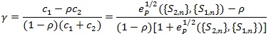
Let,  ;
;
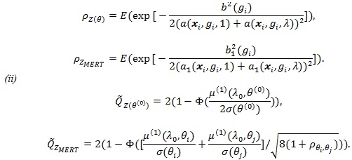
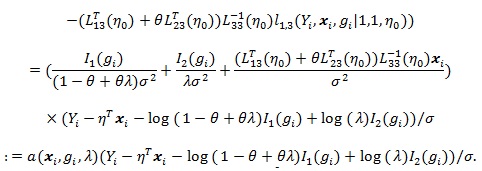
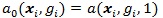
Below we give values pz(θ(0)) and pZMERT and so that their Chernoff ARE can be obtained. We also give and, so their modified Chernoff ARE can be obtained. For the chi-squared test T, under T1 its asymptotic distribution is a non-central chi-squared distribution, with a non-closed form, its modified Chernoff index is not directly computable. Let  , where g1 is the observed genotype of the i-th individual, x1 is the corresponding covariates, and let;
 |
Let,
 and
and

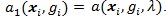
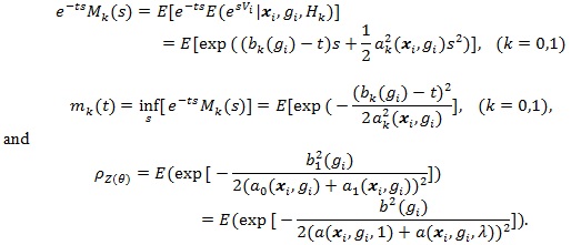
Proposition 2. (i) Assume
 is normal with mean
 and variance
 . Then, for E to denote expectation with respect to (xi, gi), we have;
 |
Hodges-Lehmann ARE. Consider testing the null hypothesis be
 given a level α test statistic Sn with critical value
 the type II error at λ is βn (λ) =
 Typically, βn (λ) tends to zero at exponential rate, the faster the better Sn is. Hodges and Lehmann (1956) [29] proposed;
 |
as a measure of the performance of Sn and it called the Hodges-Lehmann index of the statistic Sn. For two test statistics S1n and S2n for the same H 0vs,H1 with d1 (λ) and d2 (λ), the Hodges-Lehmann ARE of {S1n} relative to {S2n} at
 is defined as;
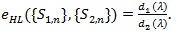 |
(14) |
For probability density functions f and g, let
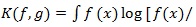 g(x]dx) be the Kullback-Leibler divergence between f) and g). For any test statistic Sn (X1,.....,Xn) based on (X1,.....,Xn) i.i.d. density
 , the Hodges-Lehmann index has the following property;
 |
and any test statistic achieve the equality in the above is said to be Hodges-Lehmann efficient.
Compared to the Pitman and Chernoff ARE, the Hodges-Lehmman ARE does not require the comparing test statistic have the same asymptotic distribution, nor they have the form of i.i.d. summations, so it has wilder application scope.
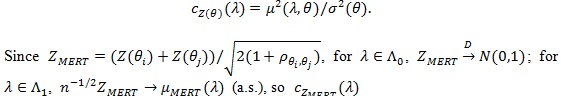
Proposition 3. Under conditions of Theorem 4 in Zheng et al. (2010) [30], with
 , given in (2), for λ > 1, we have;
 |
For the chi-squared test T, under H1 its asymptotic distribution is a non-central chi-squared distribution, with no-closed form. So its Hodges-Lehmann ARE is not directly available.
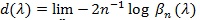
Bahadur ARE. Consider testing the null hypothesis be
Let Fn,λ(.) be the distribution function of a test statistic Sn under pλ, and for
 , let;
 |
the p-value of the observed Sn under the distribution pλ, and;
 |
if the limit exists. Typically, Ln tends to one and Ln tends to zero exponentially fast, and the faster, or the bigger c(.), the better Sn is. For two test statistics Si,n (l = 1,2) for the same hypothesis with Ln, Ci (λ), and sample size ni, to perform “equivalently” in the sense lim n1-1 log L2,n2 = lim n1-1 Log L1,n1, the Bahadur ARE of S1,n log L1n, the Bahadur ARE of relative to S2,n, at , is defined as, and has the property
 |
(15) |
The limit C can be computed under the following conditions.
(B1). For

(B2). For the interval
 , there is a function g on l, such that;
 |
(Bahadur, 1960 [13]). If Sn satisfies (B1)-(B2), then for
,
 |
For any test statistic Sn (X1,....,X2) based on X1,....,Xn i.i.d. density
 Bahadur (1967) [16] obtained the following;
 |
Note although the above relationship is regarded as a dual to that of the Hodges-Lehmann index, the two are not equivalent as
 A test statistic is said to be Bahadur efficient if for each
 limn, log

Bahadur efficiency of likelihood ratio test has been studied by a number of researchers for some special distribution families. Arcones (2005 [17], Theorem 3.3) proved that, under some regularity conditions, the likelihood ratio statistic is Bahadur efficient. Let
be the density function of the data, under his conditions of Theorem 3.3, for each fixed λ > 1 and θ, we have;
 |
Like the Hodges-Lehmman ARE, Bahadur ARE does not require the comparing test statistic have the same asymptotic distribution, nor they have the form of i.i.d. summations, so it has wide application scope.
For computation easiness, we consider a local version of Bahadur ARE. Consider testing H 0: λ = λ 0vs the local alternative H 0: λ = λ 0 + n-1/2. Let F 0 be the asymptotic distribution function of Sn under H 0, we define;
 |
Typically, 0 <
 <1. The smaller
, the better Sn is. For two test statistics Si,n(i = 1,2) for the same hypothesis with Gi,n and
<1. The smaller
, the better Sn is. For two test statistics Si,n(i = 1,2) for the same hypothesis with Gi,n and
 , we define the local Bahadur ARE of S1,n relative to S2,nas;
 |
(16) |
Proposition 4. (i) with µMERT (λ) given in Proposition 3, we have;
 |
(ii) Under conditions of Theorem 4 in ZLY, µMERT (λ) with be the derivative of µMERT (λ), θ 0 be the value of θ H 0 under, we have;
 |
4. SIMULATION AND APPLICATION TO GENETIC ASSOCIATION STUDIES
4.1. Simulation Study
Let P be the Minor Allele Frequency (MAF) of a marker of interest. We consider case-control data with r = 500 cases and s = 500 controls,
 and the disease prevalence K = 0.05. We generate 1000 datasets, and compute the means and standard deviations of
 For ZMERT, we choose θi = 0 and θj = 1.
Table T1 shows the result, the means of AREs and the standard deviations of AREs are in brackets. First we can see the mean of all three AREs are less than 1, which show that Zθo is consistent better than ZMERT. Corresponding tothis fact when θ = θ(o) is the true value Zθ(o), is asymptotically most powerful. Then the three AREs are increased with the P or λ increased. Third, the ep has the lowest variance among the three AREs, next is
 , last is

| - | - | λ - 1.1 | λ - 1.1 | λ - 1.1 | ||||||
|---|---|---|---|---|---|---|---|---|---|---|
| MAFθ0 | θ (0) | ep |  |
 |
ep | |
|
ep | |
|
| 0.15 | 1/2 | 0.874 | 0.876 | 0.827 | 0.887 | 0.904 | 0.856 | 0.895 | 0.917 | 0.869 |
| - | - | (0.056) | (0.1) | (0.115) | (0.048) | (0.084) | (0.11) | (0.039) | (0.069) | (0.097) |
| - | 1 | 0.654 | 0.814 | 0.723 | 0.654 | 0.837 | 0.746 | 0.652 | 0.85 | 0.761 |
| - | - | (0.037) | (0.094) | (0.101) | (0.031) | (0.084) | (0.094) | (0.029) | (0.075) | (0.092) |
| 0.3 | 1/2 | 0.963 | 0.94 | 0.912 | 0.97 | 0.954 | 0.929 | 0.973 | 0.961 | 0.937 |
| - | - | (0.018) | (0.05) | (0.069) | (0.013) | (0.042) | (0.064) | (0.011) | (0.039) | (0.061) |
| - | 1 | 0.73 | 0.841 | 0.751 | 0.729 | 0.853 | 0.763 | 0.728 | 0.863 | 0.775 |
| - | - | (0.03) | (0.045) | (0.056) | (0.028) | (0.043) | (0.055) | (0.025) | (0.037) | (0.05) |
| 0.45 | 1/2 | 0.991 | 0.985 | 0.978 | 0.993 | 0.986 | 0.978 | 0.995 | 0.989 | 0.983 |
| - | - | (0.006) | (0.038) | (0.055) | (0.004) | (0.036) | (0.054) | (0.003) | (0.032) | (0.051) |
| - | 1 | 0.76 | 0.85 | 0.766 | 0.758 | 0.856 | 0.771 | 0.76 | 0.861 | 0.775 |
| - | - | (0.032) | (0.033) | (0.044) | (0.031) | (0.031) | (0.042) | (0.027) | (0.028) | (0.039) |
4.2. Application
We use 6 reported SNPs associated with breast cancer 2 (Hunter et al. 2007 [31]; Li et al., 2008 [32]) to illustrate the ARE of ZMERT. These 6 SNPs are rs10510126, rs12505080, rs17157903, rs1219648, rs7696175, and rs2420946. The counts of subjects with three types of genotypes in cases and controls are shown in Table 2, where (r0, r1, r2) is the number of three genotypes in cases and (s0, s1, s2) is the number of genotypes in controls. From the table, we find three AREs of Ep, Ec and Eb are higher than 75%, sometimes it can reach 97%. For example, for SNP rs17157903, the AREs of, and are 0.8255, 0.8453 and 0.7642, respectively. It shows that ZMERT is a robust test.
| SNPid | r0 | r1 | r2 | r0 | r1 | r2 | Ep | Ec | b0 |
|---|---|---|---|---|---|---|---|---|---|
| rs10510126 | 955 | 180 | 10 | 854 | 272 | 14 | 0.8085 | 0.84 | 0.7594 |
| rs12505080 | 608 | 477 | 50 | 628 | 408 | 99 | 0.8976 | 0.8725 | 0.8202 |
| rs17157903 | 777 | 316 | 18 | 862 | 220 | 26 | 0.8255 | 0.8453 | 0.7642 |
| rs1219648 | 352 | 543 | 250 | 433 | 538 | 170 | 0.9805 | 0.9719 | 0.9585 |
| rs7696175 | 353 | 605 | 187 | 396 | 496 | 249 | 0.9686 | 0.9476 | 0.9285 |
| rs2420946 | 357 | 546 | 242 | 440 | 537 | 165 | 0.9792 | 0.9673 | 0.9512 |
APPENDIX
Derivation of
 : From (P3), we have
 . Also, as in the proof in Serfling (1980 [8], p. 317-318),
 if and only if
 |
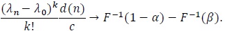
Thus, for βi,n (θ n) → β, we must have;
 |
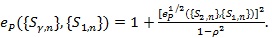
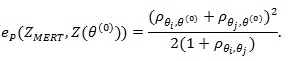
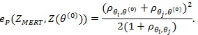
Proof of Proposition 1: We use (4) to compute ep (ZMERT,Z(θ(0))). By definition of Z(θ(0))) and CLT we have
 , and by Theorem 3 in ZLY,
 Also Z(θ(0))), and ZMERT)are jointly asymptotic normal with correlation
 . Thus the condition of (4) are satisfied, and it gives;
 |
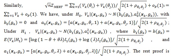
Proof of Proposition 2. (i) By assumption
 As in the proof of Theorem 4 in ZLY, we have that
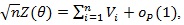 where the Vi = Vi (θ) ’s are i.i.d. with;
 |
 |
Under
 with
with
 and
and
 Under
Under
 with
with
 and
and
 So we have
 |
 |
By example A in Serfling (1980 [8], p. 330), we have;
 |
 |
similar to that for (Z(θ(0))).
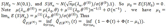
(ii). We first compute
 . In this case, let be the weak limit of (Z(θ(0))). Then,
 |
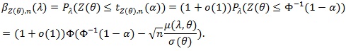
Proof of Proposition 3. Since under
 , we have tn(α)→ Ф-1 (1- α); and under
 is continuous on (- ∞, ∞), the distribution function of
 converges to uniformly Ф (.). Note µ(λ, θ) > 0, so for λ > 1 we have;
 |
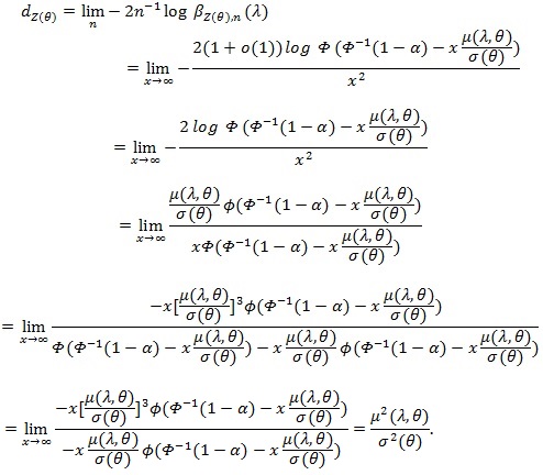
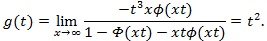
Let
 , using L’hopital’s rule twice, we get;
 |
Similarly, under
 where
where
 The same way we get;
 |
Proof of Proposition 4. i). In our case
 and when
 uniformly in Sn. From proof of Theorem 4 in ZLY, we have that for
 (a.s.). Now we compute, for

 |
Let
, and use L’Hopital’s rule,
 |
Since
 , and by L’hopital’s rule,
 , so use L’Hopital’s rule on the above again,
 |
Thus by Bahadur’s (1960) [13] Theorem,
 |
is similarly computed;
 |
Similarly, under
 , (a.s.), so
 |
CONSENT FOR PUBLICATION
Not applicable.
CONFLICT OF INTEREST
The authors declare no conflict of interest, financial or otherwise.
ACKNOWLEDGEMENTS
Declared none.