RESEARCH ARTICLE
Consistency of the Kaplan-Meier Estimator of the Survival Function in Competiting Risks
Didier Alain Njamen Njomen1, *, Joseph Wandji Ngatchou2
Article Information
Identifiers and Pagination:
Year: 2018Volume: 9
First Page: 1
Last Page: 17
Publisher Id: TOSPJ-9-1
DOI: 10.2174/1876527001809010001
Article History:
Received Date: 23/11/2017Revision Received Date: 26/02/2018
Acceptance Date: 25/03/2018
Electronic publication date: 30/04/2018
Collection year: 2018
open-access license: This is an open access article distributed under the terms of the Creative Commons Attribution 4.0 International Public License (CC-BY 4.0), a copy of which is available at: https://creativecommons.org/licenses/by/4.0/legalcode. This license permits unrestricted use, distribution, and reproduction in any medium, provided the original author and source are credited.
Abstract
Introduction:
In this article, we only focus on the probability distributions of the breakdown time whose causes are known, and we consider a partition of the observations into subgroups according to each of the causes as defined in Njamen and Ngatchou [1]. By adapting the stochastic processes developed by Aalen [2, 3], we derive a Kaplan-Meier [4] nonparametric estimator for the survival function in competiting risks.
Result & Discussion:
In a region where there is at least one observation, we prove on one hand that this new nonparametric estimator is unbiased in competiting risk and on the other hand, using the Lenglart inequality, we establish its uniform consistency in competiting risks.
1. INTRODUCTION
1.1. Analysis of Survival Times
The main source of difficulty in survival analysis, and for various reasons, is the presence of missing data. For such observations, conventional statistical procedures are no longer valid and more sophisticated statistical tools are used to model such an observations in order to validate the experimental results. The left truncated data model experimental designs frameworks for life times that have to be “large enough” to be observed. Indeed, the life time lenght T must be greater than a truncation variable Y to be observed. Thus, observations are possible only if T ≥ Y. It is a model that first appeared in astronomy, where samples are compound by astral objects from a certain area. The absolute and apparent luminosities of an astral object are respectively defined as its observed brightness at a fixed distance and from the Earth and one observe only objects that are bright enough, that is those for which the luminosity M ≥ m, are so-called left truncated data, where m is the truncation variable. In that case, we have N objects in the sample, but we are able to observe only the n objects sufficiently brilliant.
The other classical case of missing data is the so-called censored data on the right. This phenomenon of censorship models experimental studies for certain diseases where patients can be lost to follow-up after a move or a non-inherent death as a road accident. As an example, let us also analyze the reliability function of a machine M In this perspective, the observation will concern the study of how n identical machines to M work and we will denote T1,...,Tn the lifetimes of these machines. These (random) variables will be assumed to be positive and from the same density f function. The corresponding cummulative distribution function will be denoted F and the reliability function will be
 |
This is a classical problem which is a focus for example to the automobile industry when it seeks to predict the lifetime of a model. In a simplified framework where all lifetimes are observed, this problem admits elementary and natural solutions. Natural and empirical estimators exist for the distribution function, for the survival function denoted by S and for the cumulative hazard rate Λ = -log(S) which are respectively the empirical survival function for S and the Nelson-Aalen estimator for Λ.
We are particularly interested in the more realistic framework where the observation of T1,...,Tn is missing. Let us illustrate this problem with the following example. In an ideal setting, an automobile manufacturer, if he insures maintenance of its vehicles, can observe the moment of the first failure of each vehicle of a model that he sells. Therefore, he can easily determine if that model is reliable. More realistically, it may happen that the first failure of certain vehicles can not be observed for various reasons (sale by certain owners, accidents independent of the performance of the vehicle, ...). In that case, one talk about a censored model: i.e; to each vehicle i,i = 1,2,...,n is associated a pair of random variables (r.v.) (Ti, Ci) of which only the smallest one is observed, Ti is the moment of breakdown and Ci is the instant of censure.
The estimation of certain functions of this model is a much more sensitive time . To solve it, denote (Y1δ1), (Y2δ2),..., (Ynδn) the observed sequence where, for all 1 ≤ i ≤ n,
 |
Here Yi is the observed time and δi is a binary variable representing the nature of this duration which takes the value 1 if it is a true lifetime and 0 if it is a censorship.
It was only after the article of Kaplan and Meier [4], that Censored data have found the relevance that is theirs in reality.
Articles and manuals dealing with censored data are several and generally use one or other of the two very different approaches: either the methods of classical statistics (Bailey [5], Kalbfleich and Prentice [6], Cox and Oakes [7], Moreau [8], Bretagnolle and Huber [9], often using combinatorial cases as in Guilbaut [10], either the one-time processes as Gill [11], Andersen and Gill [12], Harrington and Fleming [13], Gross and Huber [14].
The nonparametric estimator of Kaplan and Meier (KM) of the survival function S is defined, in the case of non-exequal, by
 |
where Y(1), Y(2),...,Y(n) are the ordered values of Y(1) and for each of the values δi is the corresponding indicator function.
This estimator has similar properties to those of the empirical distribution function, in particular, it verifies a global asymptotic normality theorem (Breslow and Crowley [15],). But it has also other properties which are typical of the presence of censorship and have the interest of giving ideas when trying to construct other estimation procedures in the presence of censorship. Breslow and Crowley [15] were the first to discuss its convergence and its asymptotic normality. For more details, see Shorack and Wellner ([16], p.304).
1.2. Competiting Risks Model
1.2.1. Introduction
The model of competiting risks have been widely studied in the literature, see e.g. Tsiatis [17], Elandt-Johnson and Johnson [18], Andersen and al [19], Crowder [20]. Competiting risks problems are often formulated in terms of potential or latent failure times corresponding to the different failure types. Let m be the number of risks acting on the population. For j = 1, let Tj be the r.v. representing the lifetime of an individual exposed to the risk of death from cause j only. We assume that the Tj are proper, so that even in the absence of any other risk, an individual will experience an event of cause j eventually. The random variables (T1,...,Tm) are called the net lifetimes corresponding to the m postulated possible causes of failure. We assume that each failure is due to a single cause and that the occurrence of an event of a given type precludes the other events from occurring. Consequently, for each individual, we cannot observe (T1) jointly but only the smallest Tj. For each individual, the observable r.v. consists of the overall failure time T and the cause of failure C.
The independent risks model postulates that the Tj are stochastically independent of each other. Several authors have shown that based on data from competiting risks, the assumption of independence of the different risks is not testable because there is no way to distinguish between independent or dependent latent lifetimes. Tsiatis [17], showed that without the hypothesis of independence of the different risks, the model of latent lifetimes is unidentifiable. Indeed, the set of crude distribution functions is consistent with an infinity of joint distributions of latent lifetimes. To each dependent-risks model, there corresponds a unique independent-risks model with the same subdistribution functions. But each independent-risks model has a whole class of satellite dependent-risks models. When the risks are dependent, Klein and Moeschberger [21] showed that the product-limit estimator for the marginal distribution function pertaining to a given risk converges with probability one to a function which may not be the same as the marginal function of interest.
Historically, the main aim of competing risks was seen as the estimation of the marginal distributions. This consists of taking data in which the risks act together and trying to infer how some of them would act in isolation i.e. to make inference free of the “nuisance” aspects. This is an attempt to make inference about the net risks from observations on the crude risks. It amounts to deriving the Fj from the observations of (T, C) This approach is justified if the independence of the risks can be assumed. Otherwise, the counter-argument is that the Fj do not describe events that physically occur, they only describe failures from some isolated cause in situations in which all the other risks have been removed somehow. If the risks are dependent, it is the cause-specific distribution function Fj, not the net distribution function Tj, that is relevant to the real situation describing failures from cause j that can occur in the presence of all the other risks. Prentice and al [22]. emphasized these points in their criticism of the traditional approach of competiting risks. Cause-specific subdistribution functions are the basic estimable quantities in the dependent competiting risks framework. But this does provide no information about the joint distribution of the lifetimes.
1.2.2. Methods for Analyzing Survival Data in Competiting Risks
Consider a population in which each subject is exposed to m mutually exclusive competing risks which may be dependent. For j {1,...,m}, the failure time from the j-th cause is a non-negative random variable (r.v.) Tj. The competiting risks model postulates that only the smallest failure time is observable, it is given by the r.v. T = min(T1,...,Tm) with distribution function (d.f.) denoted by F. The cause of failure associated to T is then indicated by a r.v. C which takes value j if the failure is due to the j-th cause for a j
 {1,...,m} i.e. if T = Tj. We assume that T is, in its turn, at risk of being independently right-censored by a non-negative r.v. C with d.f. G. Consequently, the observable r.v. is
 |
where δ(.) denotes the indicator function. As T and C are independent, the r.v. Z has d.f. H given by 1 - H = (1 - F)(1 - G). Let τH = sup{t:H(t) < 1} denotes the rightendpoint of H beyond which no observation is possible. The subdistribution functions F(j) pertaining to the different risks or causes of failure are defined for j {1,..,m} and t ≥ 0 by
 |
For t ≥ 0, the quantity F(j)(t) represents the probability that an event of type j will occur before time t and that the other types of event have not yet occurred at this time. The functions F(j) are improper distribution functions since they are not worth 1 at infinity, i.e. limt → ∞ F(j) (t) < 1.
When the independence of the different competiting risks may not be assumed, the functions F(j) for j {1,..,m} are the basic estimable quantities.
In this paper, we are interested supplying the consistency of the nonparametric Kaplan-Meier estimator of the survival function Sj = 1 - F(j) for j = {1,...,m}in the presence of independent right-censoring in a context of competiting risks.
The Kaplan-Meier estimator was developed for situations in which only one cause of failure and the independent right-censoring are considered. Aalen and Johansen [23] were the firsts to extend the Kaplan-Meier estimator to several causes of failure in the presence of independent censoring. In the present situation, the d.f. F may be consistently estimated by the Kaplan-Meier estimator denoted by  . For j
 {1,..,m}, the subdistribution functions F(j) may be consistently estimated by means of the Aalen-Johansen estimators denoted respectively by
  , hence the nonparametric estimator of the survival function
  = 1 -
= 1 -  for j
for j {1,..., m}. Indeed, when the process of the states occupied by an individual in time is a time-inhomogeneous Markov process, Aalen and Johansen [23] introduced an estimator of the transition probabilities between states in presence of independent random right-censoring. The competiting risks set-up corresponds to the case of a time-inhomogeneous Markov process with only one transcient state and several absorbing states (that can be labeled 1, ..., m).
2. PRELIMINARY RESULTS
Throughout this section, we recall some notions of literature that will be useful for the future and that will allow a good understanding of this paper. Indeed: firstly, we recall the analysis of life-duration data in the classical case (see Bailey [5], Kalbfleich and Prentice [6], Cox and Oakes [7], Moreau [8], Bretagnolle and Huber [9], Guilbaut [10], Gill [11], Andersen and Gill [12], Harrington and Fleming [13], Gross and Huber [14]...); in a second case, we recall the estimation of the data analysis of lifetimes in competitive risks that we use in this paper (see Njamen and Ngatchou [1], Tsiatis [17], Anderson et al. [19], Moeschberger and Klein [21], Prentice and al [22], Aalen and Johansen [23], Njamen [24]...).
2.1. Choice of Censorship
We work within the framework of a right random censorship:
Definition 1 Given an - sampleT1,...,Tnof a positive random variable T. We say that there is random censorship of this sample if there is an-dimensional random variable (C1,...,Cn) such that, rather than observingT1,T2,...,Tn we observe
 |
(1) |
where Yi is the time actually observed.
Moreover, what is the nature of this duration: if δi = 1, it is a survival, if δi = 0, it is a censorship.
Example 1 During a biological experiment, we are interested in the cause of death that takes place after a period of timeT that we wish to study the law, but another cause of death may occur before and thus prevent the observation of T by a right censorship. The usual hypothesis, which allows us to carry out the calculations, is the independence of T and C. This hypothesis has been relaxed by Jacobsen [25]. We notice, however, that if we allow a dependence betweenT and C, the same law of the couple (Y C, 1T≤C) can come from several marginal laws different forT and C, which have as a consequence a problem of identifiability.
The distribution of T is entirely characterized by five functions: cumulative distribution function, probability density function, survival function, hazard function, cumulative hazard function (or integrated). Let (Ω,A, ) be a probability space.
2.2. Identifiability Problem in a Censorship Model
Consider the censorship model defined by (1). If we know the law of observation of Y, can this allow to identify the exact law of the variable of interest T ? In other words, if we knew perfectly the law of observations, could we deduce the unique law of T (for example, its density function or its survival function)? It’s not always possible, because the fact of having missing data implies a loss of information.
In general, if durations and censures are not independent, it is not possible to identify the law of T from the observations. On the other hand, when durations and censures are independent, identification is possible.
For any cumulative distribution function L, we denote by τH = sup {t:L(t) < 1}.
On the other hand, Ln(.) shall designate a functional estimator of Ln(.). Finally,  (.) = 1 - L (.).
Proposition 1 In the case of a random right censorship C, if T and C are independent with cumulative distribution function F and G respectively and if τF ≤ τG , then the law of T is identifiable from the law of the observations (Yi, δi).
Proof See Fermanian [26, p.11].
Remark 1 The hypothesis of independence between duration and censorship is not always realistic. In the case of right censorship caused by the end of the survey process, it is natural. But when somebody is exposed to several risks of death (in the case of competiting risks), it could be questionable: these risks are all dependent on the general state of health (for example, vascular tension). A particular risk (for example, a heart attack) is likely to be correlated with others (for example, a stroke) which, if they arise, censor it eventually.
2.3. Classical Case: Estimation of Survival Function
Let (Ω,A, ) probability space.
Let T1,...,Tn be a sequence of real random variables of interest independent and identically distributed (i.i.d.) of common cumulative distribution function F and of probability density f. Let C1,...,Cn be a sequence of random variables of censures i.i.d. of the continuous cumulative distribution function (c.d.f.) G. The Ci are also assumed to be independent of the Ti.
Let {(Y1, δ1)...(Yn, δn)} be the observed sample defined by (1). The (Yi)i are (c.d.f.), H is given by
 |
Let H1 and H0 be the (c.d.f.) of uncensored and censored random variables (r.v.).
 |
and
 |
We have the identity
 |
By classifying the (Yi) in ascending order, one obtains the statistic’s order
 |
Denote Ii = [Y(i-1), Y(i)]. The non-parametric Kaplan-Meier (KM) estimator for survival function (s.f.) is also called PL (Product-Limit) estimator because it appears as the limit of a product. This estimator is interested in estimating the quantities of the form:
 |
where pi is the probability of surviving during the interval Ii, when one is living at the beginning of this interval, then qi = 1 - pi = probability of dying during this interval knowing that one was living at the beginning of this interval.
We now define the concept of a risky subject in order of getting its natural estimator of qi.
Definition 2 (Subject at risk) At each instant, we define the numberZn(t) of the subjects at risk as the number of subjects present (i.e. neither dead nor censured) to t-
 |
Let us denote by  the number of uncensored observations that are less than or equal to the instant t, i.e.
 |
Therefore a natural estimator of qi is
 |
2.3.1. Expression of the Empirical Survival Function
If the data is not censored, Sn(t) can be estimated by the c.d.f.
 |
(2) |
where Fn(t) is the empirical c.d.f. of Ti. If observations (Ti) with censures are available, estimate S only by the data (Ti), i = 1,...,n uncensored (δi = 1) provides a biased estimate. Indeed if we define an estimator  ,
,
 |
(3) |
then by the law of large numbers we have:
 |
(4) |
because
 |
Thus, in the case of censored data, the estimation of the survival function S requires specific tools. There are several non-parametric methods among which the well known is the one of Kaplan-Meier. First, we define the non-parametric estimator of the survival function, which can be deduced immediately from the estimation of cumulative risk function, also called the cumulative hazard rate Λ, defined by Λ(t) =  .
.
2.3.2. Nonparametric Estimator of the Survival Function
By the relationship = exp(-Λ) and by estimating Λ by the Nelson-Aalen estimator  defined in Njamen and Ngacthou [1], We obtain the non-parametric estimator of the survival function of S given by:
 |
(5) |
It can also be written as the following:
 |
where m(ti) denotes the number of “events” observed up to the moment ti and r(ti) is the number of “individuals” at risk at time ti
2.3.3. The Estimator of Kaplan-Meier (KM) [4]
In 1958, Kaplan and Meier proposed an estimator of the survival function S, also called a product-limit estimator. It is based on the following idea: an “individual” is alive after the instant t means to be alive just before the instant t and not to “die” at t.
Definition 3 At any point, the estimator of KM of the survival S of the lifetime variable Ti is, with the above definitions:
 |
(6) |
with  .
.
If there is no ex-aequo (i.e. identical death times for several subjects), we can simply write  (t) in the following form:
 |
(7) |
The Kaplan-Meier non-parametric estimator Gn of G is obtained as the following:
 |
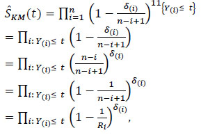
Let T(1) ≤...≤T(n) be the associated statistics order, then the Kaplan-Meier estimator defined in (7) is rewritten for all t by
 |
(8) |
where Ri = n-i + 1.
The identity (8) comes from the following property:
 |
The Kaplan-Meier non-parametric estimator is widely used in several fields in the society (demography, actuarial science, psychology, etc.) and in the basic sciences, particularly in epidemiology, to show the effectiveness of a treatment compared to another one.
2.3.4. Examples of Analysis of Censored Data by the Kaplan-Meier Estimator
Example 2 (Friereich and et al.,[27]) In 1963, Freireich et al. conducted a therapeutic trial to compare the remission durations in weeks of leukemia according to whether they received 6-mercaptopyne or placebo (The control group received placebo and the trial was double-blind).
Remission duration, in the week, according to treatment:
 |
The numbers followed by the sign + correspond to patients who were lost of sight or “censored” on the date considered. They are therefore excluded “alive” from the study and we know only from them that their survival duration is greater than the one indicated. For example, the fourth patient treated with 6M-P had a remission duration of more than 6 weeks.
The calculations give us:
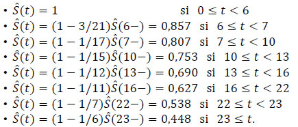 |
The Kaplan-Meier method consists of estimating the survival probability over a period of time, in other words, the probability of being alive at the end of the interval if we were at the beginning of the interval. Therefore it is necessary to calculate the number of patients presenting the event in this interval divided by the number of patients exposed to the risk of the event during this interval.
Tables 1 and 2 provide general information about the two treatments.
| t=6MP | ||||||
|---|---|---|---|---|---|---|
| Time | N.risk | N.event | Survival | Std.err | Clower 95%CI | Upper 95%CI |
| 6 | 21 | 3 | 0.857 | 0.0764 | 0.720 | 1.000 |
| 7 | 17 | 1 | 0.807 | 0.0869 | 0.653 | 0.996 |
| 10 | 15 | 1 | 0.753 | 0.0963 | 0.586 | 0.968 |
| 13 | 12 | 1 | 0.690 | 0.1068 | 0.510 | 0.935 |
| 16 | 11 | 1 | 0.627 | 0.1141 | 0.439 | 0.896 |
| 22 | 7 | 1 | 0.538 | 0.1282 | 0.337 | 0.858 |
| 23 | 6 | 1 | 0.448 | 0.1346 | 0.249 | 0.807 |
| t = P | ||||||
|---|---|---|---|---|---|---|
| Time | N.risk | N.event | Survival | Std.err | Clower 95%CI | Upper 95%CI |
| 1 | 21 | 2 | 0.9048 | 0.0641 | 0.78754 | 1.000 |
| 2 | 19 | 2 | 0.8095 | 0.0857 | 0.65785 | 0.996 |
| 3 | 17 | 1 | 0.7619 | 0.0929 | 0.59988 | 0.968 |
| 4 | 16 | 2 | 0.6667 | 0.1029 | 0.49268 | 0.902 |
| 5 | 14 | 2 | 0.5714 | 0.1080 | 0.39455 | 0.828 |
| 8 | 12 | 4 | 0.3810 | 0.1060 | 0.22085 | 0.657 |
| 11 | 8 | 2 | 0.2857 | 0.0986 | 0.14529 | 0.562 |
| 12 | 6 | 2 | 0.1905 | 0.0857 | 0.07887 | 0.460 |
| 15 | 4 | 1 | 0.1429 | 0.0764 | 0.05011 | 0.407 |
| 17 | 3 | 1 | 0.0952 | 0.0641 | 0.02549 | 0.356 |
| 22 | 2 | 1 | 0.0476 | 0.0465 | 0.00703 | 0.322 |
| 23 | 1 | 1 | 0.0000 | NA | NA | NA |
The two tables above, obtained from the R code > summary(s), allow us to have not only the survival of all the events at risk, but also Greenwood’s approximations of the variance of survival, as well as the confidence interval in the survival curve.
The following graphs, obtained by the R software, allow us to compute the curve of treatment with 6-mercaptopuria and the curve of treatment with Placebo.
Figs. (1 and 2) represent respectively the survival curve with the evolution of the number of patients at risk during the follow-up, whose the survival curve is the graphical representation of the survival function, i.e. the probability of survival as a function of time. At the beginning of each curve, 100% of patients are alive (probability 1), it’s a stepped curve with a step corresponding to each event. The height of the step is proportional to the number of events on the interval. The lost-of-view is represented by vertical bars throughout the step of the staircase. If the censors are too many and taint the graph, they are not respected, which is not the case for the two graphs above. The accuracy of the estimation of those survival curves Figs. (1 and 2) is represented by a confidence interval of 95%. This interval takes the form of two curves corresponding to the upper limit and the lower limit (see in the dashed lines in the graphs above). This interval has a probability of 95% to include the true survival curve. The two survival curves above are under the form of steps, continuous by lump and jumps at each point of discontinuity.
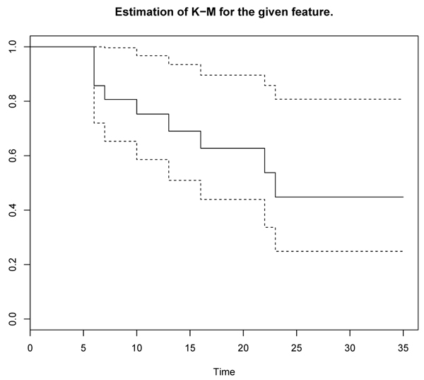 |
Fig. (1). Estimation of K-M for 6-mercaptopurnie. |
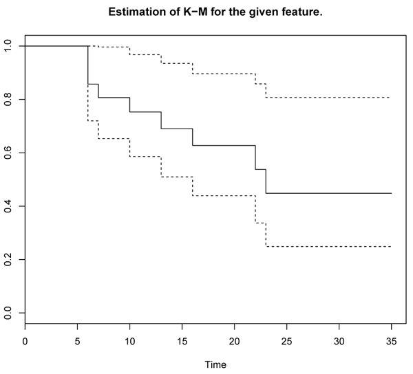 |
Fig. (2). Estimation of K-M for Placebo. |
These two curves can also be obtained in the same graph, which will make it possible to obtain a more precise and concise analysis:
Note that Fig. (3) graph above contains two curves representing the follow-up of treatment with by 6-mercaptopurine and placebo treatment. This graph is obtained by software R. These are staircase curves with the corresponding margin for each event. The height of the margin is proportional to the number of events on the interval. The lost-of-view is represented by vertical bars throughout the staircase. These two survival curves are in the form of a staircase, continuous by piece and have jumped at each point of discontinuity. Finally, we note that the 6-MP treatment curve is higher than that of the Placebo effect. Hence the 6-MP treatment effective.
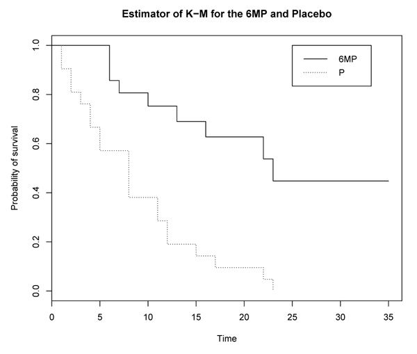 |
Fig. (3). Curve of K-M of the survival function for Freireich data. |
2.3.5. Properties of the KM Estimator in the Classical Case
The asymptotic properties of the KM estimator have been studied by several authors (see e.g Peterson [28], Andersen et al. [19], Shorack and Wellner [16]). A consistency property of the KM estimator is given by:
Theorem 1 If the survival T of the distribution function F and the censure C of the distribution function G are independent, then
 |
Proof See Shorack and Wellner ([16], p. 304).
The first strong representation of Fn-F by an average of v.a. i.i.d. was obtained by Burke and et al [29, 30], with a remainder of order O(n-1/2logn2n). This result is based on the work of Komlos, et al. [31], on the approximation of empirical processes. A second type of approximation was established by Lo and Singh [32], with a negligible term of order O((n-1logn)3/4). This rate was then improved to O(n-1logn) by Lo et al [33].
2.4. Case Where The Modeling is in a Contest of Competiting Risks
2.4.1. Estimation of Lifetimes in Competiting Risk
The modeling done in this work is that obtained from Njamen and Ngatchou [1]. We recall the main lines of this modeling: let τ1, τ2,...,τm be a continuons random variables representing respectively the lifetimes in each of the m risks competing, J = {1,2,...,m} {0} be the set of index cause, where 0 corresponds to the condition of the individual observed, T = min(τ1, τ2,...,τm) the random variable case, where η = j if T = τj , for all j = 1,2,...,m, F is the distribution function of T, S = 1 - F the survival function such that S(t) =
  [T > t], the random variable C of the event censoring right, δ = 11T ≤ C and for technical reasons, ξ = η δ such that ξ = j if (T ≤ C and η = j) and ξ = 0 if T > C.
We notice that δ and ξ are observable and η is so only for T uncensored.
We assume that censorship is not informative. The joint law (T,η) is completely specified by the specific incident distributions cause j ,F(j) (t) defined by
 |
(9) |
which are none other than the sub-distribution of the specific cause of failure j = 1,...,m. The cumulative hazard rate of specific-cause j (j = 1,...,m) corresponding to (1) is given by
 |
(10) |
Let (Z1, δ1, ξ1)...(Zn, δn, ξn) be n- sample of observable triplet (Z1, δ1, ξ1) where Zi = min(Ti, Ci) and δi = 11{Ti≤Ci}, which Ti = min(τi1,...,τim) and where τij represents the time that an individual i is subject to the cause j. If Ti and Ci are independent, the random variable Zi admits distribution function Hi defined by 1 - Hi = (1 - Fi) (1 - Gi). Nelson-Aalen’s estimator of Λj is given for j = 1,...,m by (see e.g in Andersen et al [19].)
 |
(11) |
which
 |
(12) |
and where
 |
(13) |
is the counting of the number of failures observed in case of j the time interval [0, t] and
 |
(14) |
is the number of individuals in sample observation that survive beyond time t. Thus, for any j {1,..,m}
 |
(15) |
The relation between the cumulative hazard rate Λ*(j) and survival S*(j) = 1 - F*(j) in the subgroup Aj is given by
 |
(16) |
is given by
 |
(17) |
Since (Zi) is a Markov process comprising a state transcendant and m absorbent states, the F(j) functions are estimable using the corresponding Aalen-Johansen [23], estimate defined for t ≥ 0 by:
 |
(18) |
where H-n is the continuous left-hand modeling of the empirical distribution function Hn defined for t ≥ 0 by
 |
The expression of the Aalen-Johansen the estimator implies equally the modification continue to the left  of Kaplan-Meier the estimator of F while is defined for all t ≥ 0 by:
 |
(19) |
The final estimator obtained for the cumulative hazard rate Λ*(j)(t) due to the specific cause j and the corresponding distribution function F*(j) (t) given by (13) and (16) are written by
 |
(20) |
and
 |
(21) |
respectively.
The relation between the Kaplan-Meier  estimator and Λ*(j)n in the context of competiting risks is given for all t ≥ 0 by:
 |
(22) |
where
 |
is a sub-distribution of Hn(t), and where for all t ≥ 0,
 |
is the Nelson-Aalen estimator for the specific cause of the cumulative hazards Λ(j).
3. MAIN RESULTS
Let T be a positive random variable and C be a censoring variable such that Z = T C and δ = 11{T≤C}. In this model of random censorship, for a sample i = 1,...,n subject to specific causes j(j = 1,...,m), we can observe the couple (Zi, δi) where Zi = min(Ti, Ci) and δi = 11Ti≤Ci with Ti = min(τi1,...,τim) and where τij is the time that an individual i is subject to the cause j.
The survival function of each individual subject to a specific cause j is defined for all j = 1,...,m by S(j) (t) = 1 - F(j) (t) =  (τj > t). So in a region where we have at least one observation, S* = 1 - F*. Applying the previous sub-section 2.4.1, we have
  (t) = 1 -
  (t) where
  (t) is the Kaplan-Meier estimator defined in Njamen and Ngatchou [1].
3.1. The Bias of the Non-Parametric Kaplan-Meier Estimator [4] on the Survival Function in Competiting Risks
The following theorem is the first fundamental result of this paper. It shows that the Kaplan-Meier nonparametric estimator [4] on the survival function possesses a bias in competing risks.
Theorem 3 The non-parametric estimator defined by
 |
(23) |
possesses a bias.
Proof
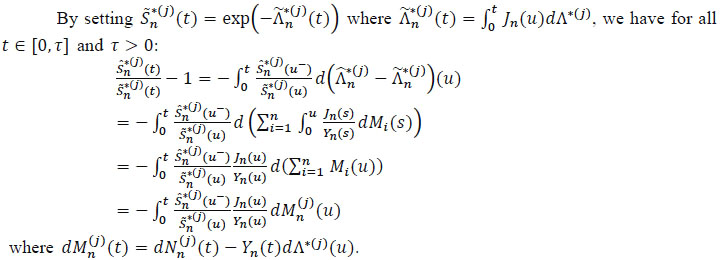 |
Since  - 1 is a local martingale of integrable square on [0, τ[ zero in t = 0 (see Lopez [34],), we deduce that:
 |
We have
 |
So
 |
and since the mathematical mean is linear, we have:
 |
From where
 |
or again
 |
Consequently, the bias is
 |
Hence the proof of the theorem.
The uniform consistency of Kaplan-Meier’s nonparametric estimator (1958) is given in the following subsection:
3.2. Uniform Consistency of the Kaplan-Meier Nonparametric Estimator of the Survival Function in Competing Risks
The following theorem is the second fundamental result of this paper. It gives the uniform consistency of Kaplan-Meier’s nonparametric  of the survival S*j in a region where there is at least one observation:
Theorem 4 If for t > 0,F*(t), < 1 and  , then for j ∈ {1,...,m}
 |
(24) |
Proof For all j {1,...,m} the nonparametric estimator of Kaplan-Meier [4] verifies
  (s) = 1 -
  (s) where
  is defined by
 |
Thus, to show that
 |
It is sufficient to show that
 |
To achieve this, we have by hypothesis t > 0,F*(t), < 1 and  . By Theorem 3.2.3 p.97 of Fleming and Harrington [35], we have:
 |
where
 |
It is sufficient to show that
 |
to have
 |
By the inequality of Lenglart, for positive η and ε and for all j = 1,...,m we have:
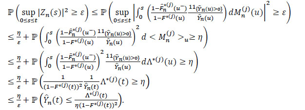 |
On the other hand,
 |
hence
 |
As ε and η are arbitrarily chosen, it is deduced that
 |
Therefore
 |
Hence the result.
CONCLUSION
In this paper, we first show that the nonparametric Kaplan-Meier estimator of the survival function has a bias in competing risks, and in a second step, we have established its uniform consistency.
CONSENT FOR PUBLICATION
Not applicable.
CONFLICT OF INTEREST
The author declares no conflict of interest, financial or otherwise.
ACKNOWLEDGEMENTS
The first author would like to thank Prof. Célestin NEMBUA CHAMENI and Kossi Essona GNEYOU for their advice and encouragements. Furthermore, The authors wish to thank the anonymous referee for the through reading and suggestions that will help to improve the paper.
REFERENCES
| [1] | Njamen DA, N. Wandji J. Nelson-Aalen and Kaplan-Meier estimators in competing risks. Appl Math (Irvine) 2014; 5(4): 765-76. |
| [2] | Aalen OO. Nonparametric estimation of partial transition probabilities in multiple decrement models. Ann Stat 1978; 6(3): 534-45. |
| [3] | Aalen OO. Nonparametric inference for a family of counting processes. Ann Stat 1978; 6(4): 701-26. |
| [4] | Kaplan EL, Meier P. Nonparametric estimation from incomplete observations. J Am Stat Assoc 1958; 53(282): 457-81. |
| [5] | Bailey KR. The general maximum likelihood approach to the Cox regression model Ph.D. Dissertation, University of Chicago, Illinois. |
| [6] | Kalbfleisch J, Prentice R. The statistical analysis of failure time data John wiley, New-York, 1980. |
| [7] | Cox D, Oakes D. Analysis of survival data, Chapman and Hall, London, 1984. |
| [8] | Moreau T. Introduction à l’étude pratique des données de survie Séminaire de statistique médicale, Université Paris V, 1984. |
| [9] | Bretagnolle J, Huber C. Effect of omitting covariates in Cox’s model for survival data. Scand J Stat 1988; 15: 125-38. |
| [10] | Guilbaut O. Exact compensations for left truncation and/ or right censorship in Kolmogorov- type tests. Research report Department of Statistics, University of Stocholm, 1987. |
| [11] | Gill R D. Censoring and Stochastic Integrals Mathematical Centre Tracts, 124 : Amesterdam: Mathematishe Centrum, 1980. |
| [12] | Andersen P, Gill R. Cox’s regression model for counting processes: A large sample study. Ann Stat 1982; 10: 1100-20. |
| [13] | Harrington DP, Fleming TR. A class of rank test procedures for censored survival data.Biometrika 1982; 10: 553-66. JSTOR |
| [14] | Gross G, Huber C. Matched pair experiments: Cox and maximum likehood estimation. Scand J Stat 1987; 14: 27-41. |
| [15] | Breslow N, Crowley J. A large sample study of the life table and product-limit estimates under random censorship. Ann Stat 1974; 2: 437-53. |
| [16] | Shorack GR, Wellner JA. Empirical processes with applications to statistics 1986. |
| [17] | Tsiatis A. A nonidentifiability aspect of the problem of competing risks. Proc Natl Acad Sci USA 1975; 72(1): 20-2. |
| [18] | Elandt RJ, Johnson NL. Survival models and data analysis John Wiley and Sons, New York, 1980. |
| [19] | Andersen PK, Borgan Ø, Gill RD, Keiding N. Statistical Models based on Counting Processes Springer Series in Statistics, Spring-Verlag, New York, 1993. |
| [20] | Crowder MJ. Classical competing risks. CRC Press, 2001. |
| [21] | Moeschberger ML, Klein JP. Consequences of departures from independence in exponential series systems. Technometrics 1984; 26(3): 277-84. |
| [22] | Prentice RL, Kalbfleisch JD, Peterson AV Jr, Flournoy N, Farewell VT, Breslow NE. The analysis of failure times in the presence of competing risks. Biometrics 1978; 34(4): 541-54. |
| [23] | Aalen OO, Johansen S. An empirical transition matrix for non-homogeneous Markov chains based on censored observations. Scand J Stat 1978; 5(3): 141-50. |
| [24] | Njamen DAN. “Convergence of the Nelson-Aalen Estimator in Competing Risks”, Int. J. Stat. Probab.. Canadian Center of Science and Education 2017; 6(3): 9-23. |
| [25] | Jacobsen M. Right censoring and martingale methods for failure time data. Ann Stat 1989; 17: 1133-56. |
| [26] | Fermanian JD. Modèles de durées Cours ENSAE 3ième année, 2005. http://www.crest.fr/ses.php?user=2975 |
| [27] | Freireich J. Emil, Gehan, and al. “The effect of 6-mercaptopurine on the duration of steroid-induced remissions in acute leukemia: A model for evaluation of other potentially useful therapy. Blood 1963; 21(6): 699-716. |
| [28] | Peterson JL. Petri nets. ACM Comput Surv 1977; 9(3): 223-52. CSUR. |
| [29] | Burke MD, Csörgõ S, Horvarth L. Strong approximation of some biometric estimates under random censorship. Z Wahrsh View Gebiete 1981; 56: 87-112. |
| [30] | Burke MD, Csörgõ S, Horvarth L. A correction to improvmement of strong approximation of some biometric estimates under random censorship. Probab Theory Relat Fields 1986; 79: 51-7. |
| [31] | Kolmos J, Major P, Tusnady G. Weak convergence and embedding limit theorems of probability theory Colloq Math Soc Janos Bolyai, North Holland 1975; 11: 149-65. |
| [32] | Lo H S. The product-limit estimator and bootstrap: some asymptotic representation Probab Theory Relat Fields 1986; 71: 455-65. |
| [33] | Lo HS, Mack YP, Wang JL. Density and hazard rate estimation for censored data via strong representation of the Kaplan-Meier estimator. Probab Theory Relat Fields 1989; 80: 461-73. |
| [34] | Lopez O. Réduction de dimension en présence de données censurées. Thèse de Doctorat Ph.D. Université de Rennes 1, No. 3640, France, 2007. |
| [35] | Fleming TR, Harrington DP. Counting processes and survival analysis John Wiley & Sons, Inc., New York, 1991. |


 . Asn→ ∞ we have:
